An Apple Pie From Scratch, Part VIIc: Geology and Landforms: Constructing Global Terrain

We have come at last to a moment I’m sure many of you have been waiting for: It’s time to take all that we’ve learned about tectonics, geology, and landform evolution and actually apply it to creating topographic maps of our worlds.

There are a few different ways to approach this, and I’ve even seen people get some success just drawing out topography by hand, but I can tell you from personal experience that it takes a long damn time to do that, and it can also be difficult to create globally consistent maps that way. Instead, I’m going to use a couple of software tools to help us along and cut out a lot of the tedium. All these software tools are freely available online.

To be clear, this post is going to be more art than science. I certainly want realistic terrain, but none of the tools available are capable of completely simulating all the processes that produce it, and even if they were, the complexity of the inputs they’d require would be well beyond what we could reasonably produce by hand. As such, the methodology I’m going to lay out is not necessarily the one and only way to produce geologically realistic maps, and altering the process to produce outputs you think look better is very much encouraged. Indeed, much of this post won’t be so much a step-by-step guide as just an overview of several available options.

Furthermore, for now this post is also something of a work in progress. The current tutorial covers producing heightmaps accounting for both tectonic action and fluvial erosion in either wilbur or gospl, but there are a few other steps I still want to add to the process that are a bit trickier to figure out:

• Accounting for glacial action (mostly in terms of large-scale subsidence and rebound) in both Wilbur and gospl.
• Allowing for the formation of endorheic basins and possibly lakes in Wilbur.
• Detecting basins on the resulting heightmaps and filling them with appropriately sized lakes based on climate data.
• Final touchups to account for coastal erosion.

Given how long this post has taken to make and how long these additional steps might take to figure out, I didn’t want to delay it any further. I’ll add these to this post when (if) I figure them out, and note the additions on the “Alterations to Existing Posts” page you can find in the sidebar.

• Step 1: Preparing Maps
• Reprojecting Maps
• Reassembling the World Map
• Step 2: Interpreting the Tectonic History
• Step 3: Seeding Terrain
• First Sketch
• Smoothing and Noising
• Step 4: Simulating Erosion
• Option A: Wilbur
• Wilbur Basics
• Automated Wilbur
• Wilbur Outputs
• Wilbur Extras
  
• Option B: gospl
• Installing gospl
• Windows
• OpenSUSE
• Preparing gospl Inputs
• Using gospl
• gospl Extras
• Step 5: Postprocessing
• Notes
  

Back to Part VIIb

Step 1: Preparing Maps

First off, you’ll want to gather together all the necessary information on your world’s geography, geology, and climate. In this case I’m drawing on the tectonic history I sketched out in Part Va and the climate I simulated in ExoPlaSim in the Part VI supplement, but you can of course include whatever’s appropriate to your process. These maps should all be in the same equirectangular projection at fairly high resolution (I used 3,600 by 1,800 pixels, though the previews shown here are all smaller to save a bit on bandwidth). In particular, I took 4 maps straight from GPlates:

A basic land/sea mask

A map of orogenies (colored by age), cratons, and failed rifts.

A map of LIPs (colored by age), hotspots, and hotspot paths.

A map of subduction zones and the outlines of all the constituent terranes (the continent, microcontinent, accreted island arc, and continent fragment features made in Gplates).

I’ll also add 2 more made outside Gplates:

The first-pass rough topography I made in Part Va (in shades of grey so as to be a bit more readable as a transparent overlay).

A climate map; in this case made in ExoPlaSim, a slight iteration from the version I produced in the Part VI supplement, run here at a higher resolution and with an obliquity of 28 degrees (this is actually a tad warmer than I want the final climate to be but it’ll do for a point of reference).

Reprojecting Maps

Now, I’ll get into cartography and map projections in Part VIII, but for now we have to keep in mind that no flat map is without distortion. Try to draw out a world on an equirectangular map and then project it back onto a globe (which, as a reminder, you can pretty quickly do in Gplates using the “import raster” function) and you’ll probably find that it’s oddly pinched near the poles. Even far from the poles, the distortion caused by the map projection is hard to account for: at 60° latitude, each square pixel actually represents an area of the surface that is about half as wide as it is tall (and so also has about half the area of pixels at the equator). Thus, rather than trying to draw out terrain details on a single world map, I prefer to split it into sections, reproject the world map into multiple maps that each have minimal distortion within one of those sections, draw out terrain in those maps, and then ultimately reproject them back into a single global map.

The main issue with this approach is that any features on the boundaries between the sections will be split between maps, which may make them difficult to draw properly and cause issues with our later erosion simulation, especially if there are any big river networks along the boundary. But presuming we’re mostly interested in terrain on land, we can mostly avoid this by using roughly continent-sized sections, with the boundaries in the open ocean. For Teacup Ae, I’ve divided up the world into 7 sections; 1 for each of the 6 continents and 1 for the large archipelago between Wegener and Steno:

I’ve done my best to draw the boundaries through empty areas of ocean—avoiding subduction zones and hotspot island chains where possible—but Hutton and Lyell together are simply too big to comfortably fit on a single map without significant distortion, so I’ve split them along a fairly flat and arid region, which should reduce issues that might arise from mountain ranges or river basins cutting across the boundaries. I also checked this map in Gplates to make sure the resulting sections are all roughly circular on the globe, with no parts extending too far from the center—allowing me to keep as much areas as possible in the areas at the center of each continental map that will have the least distortion.

For our map reprojection, we can use G.Projector, a free program that can reproject an input map into a bewildering number of projections (you may need a Java update to run the latest version). It can accept equirectangular maps as input, but also maps in the Hammer projection, which is a map type with fairly low distortion near its center (Aitoff might actually have a bit less, but Hammer displays areas near the center in higher detail than Aitoff, and as a nice bonus is equal-area as well; the relative area of features on the map is proportional to their area on the surface of the globe); so Hammer is a good choice for maps we want to project out to minimally distorted continent maps and then later reproject back into a single global map (even if, for reasons we’ll discuss later, you don’t use G.Projector for the latter step).

We can load each of our equirectangular maps into G.projector and reproject them into the “Hammer (oblique)” projection, which allows us to center the output map over any part of the globe. With a bit of experimentation, I’ve found a center point for each continental section that places the bulk of the main landmass near the center of the map map while making sure that none of the extreme ends are too far towards the edges. When you do this, be sure to note down the latitude and longitude of those centers, as you’ll need them for projecting each of the maps you want to use in the next steps and for reprojecting the final maps back to a single global map later.

Oblique Hammer projection centered on 120° E, 20° S to focus on the continent of Wegener.

You should export these maps with no graticules, overlay, or border—the last one in particular messes with the map scaling (as the actual map area is shrunk to fit the border). They should also have about as high resolution as you can manage; G.projector can export up to 20,000 by 10,000 pixels, though more than a few people have reported trouble getting it to work well at resolutions that high (it helps to open the program without any import first and then import a large file within the program, and it’s not unusual for the program to freeze for a few minutes when exporting a large image; if you just can't get it to export at high resolution, look into either using projectionpasta which I'll describe shortly or Map Designer) and it may make some of our editing programs struggle, so figure out which resolution works best for you.

At a guideline, the relationship between position on a Hammer projection and map scale is a little complicated, but near the center the width and height of each pixel in kilometers should be equal to about [0.9 * (planet circumference in km) / (width of map in pixels)]. For Earth at 20,000 pixels wide that’s 1.80 km/pixel, and each pixel represents 3.24 square kilometers of the surface. As you get further from the center, the width and height scale shifts—at 90° west or east each pixel is 1.95 km wide and 1.67 km tall, a ratio of 1.17—but because Hammer is equal-area, every pixel should still represent the same area of the surface.

For Teacup Ae, with a radius of 6130 km and thus a circumference of 38,516 km, a resolution of 17,300 pixels wide by 8,650 tall results in a convenient resolution of almost exactly 2 km/pixel in width and height at the center and 4 km²/pixel in area across the map (in case you're wondering, 18,000 x 9,000 would give you the same scale—to within 0.1%—for an exactly Earth-sized planet). I’ll reproject each of the maps I prepared earlier at this resolution, as well as a separate maps of graticules (lines of latitude and longitude) at 10° intervals.

Graticules map for Wegener, with a center 20° south of the equator.

And a map of the continental sections I divided the planet into, though in this case I’ve drawn them as colored sections rather than dividing lines, as those lines would get thinned out or broadened in the reprojection process in a way that would make it hard to keep track of their exact position (there’s probably a better way to save them as a shapefile and then use some other software to reproject them but I won’t overcomplicate matters here).

We can then stack these maps back together in my image editor, and to reduce the load on my computer we can then crop down each stack to just the continental area of interest. But take special care to note exactly what part of the original image you’ve cut out so that we can place it back on the full world map later. In this case, for example, I first cut away areas to the south and east of Wegener to create a map of 10800 x 7400 pixels, and then cut away areas to the north and west to get a map of 5100 x 5600 pixels.

Thus, I get 7 maps that together cover the whole surface at high resolution, but with reasonably low distortion and moderate individual file sizes. Even if you’re not going to go into any of the detailed terrain drawing and erosion simulation of the rest of the tutorial, this reprojection process is a good way to avoid the distortion issues a lot of people run into with world maps.

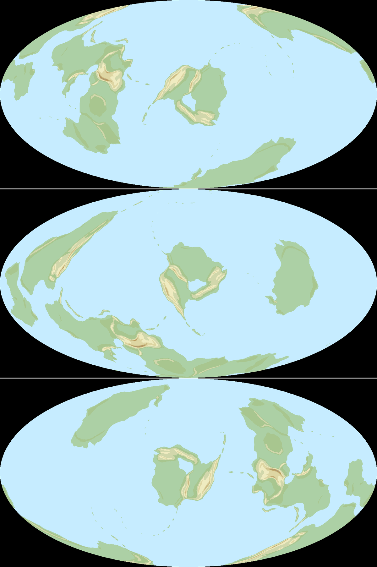
The 7 continental sections in their individual Hammer projections.

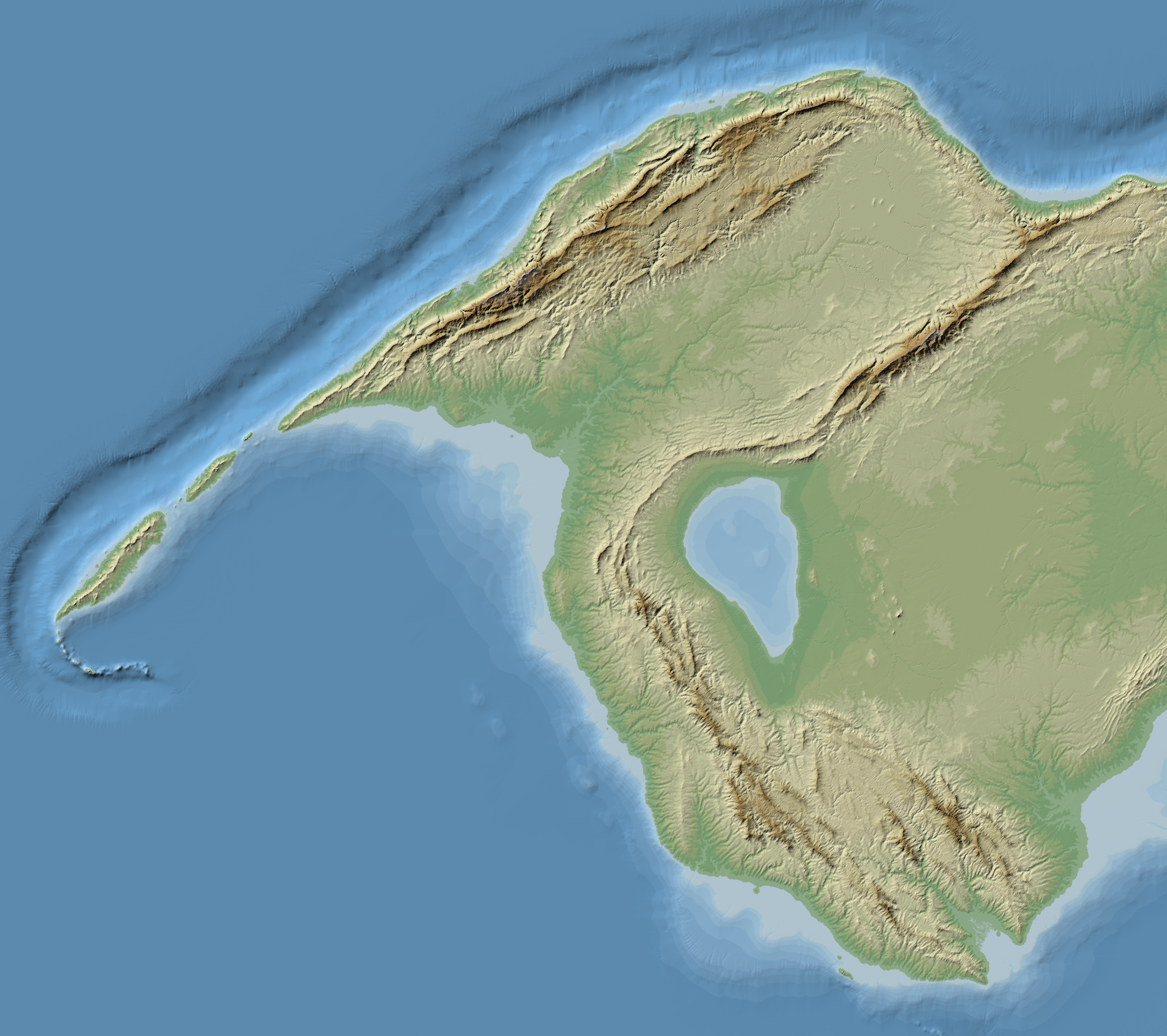
I do hope to produce terrain maps for the entirety of Teacup Ae in the near future, and I’ll make some short posts detailing some of my design choices when I do, but in the interest of brevity I’ll focus just on Wegener for the remainder of this tutorial, as it contains a pretty decent range of landforms we can use to test our methods—and I’ll particularly focus on the northwestern peninsula, which has a nice range of terrain features to use as examples.

Reassembling the world map

While we’ve got map projections on the mind, I’ll briefly skip ahead to the process for reassembling these continent maps into a single world map once we’re done with whatever we decide to do with these maps (though the individual Hammer projections may serve nicely as regional maps and I’ll probably use them as such in the future).

First off, we want to put out trimmed maps back on properly scaled world maps, which is basically just the reverse of the trimming process; most image editors have some option to increase the “canvass size” while keeping the existing image anchored to the middles, edges, or corners. With Wegener, for example, I  first I expand the map west and north to 10800 x 7400 while anchoring Wegener in the southeast corner, and then anchor that to the northwest corner and expand the map south and east to get back to 17300 x 8650.

Though G.projector can take Hammer maps as input and reproject them back to equirectangular (using the equirectangular (oblique) projection, though it would have to be done in 2 steps; in the case of Wegener, which I recentered to 120° east, 20° south, I would first have to export it in equirectangualr recentered 20° north, and then import that resulting map and export again recentered 120° west; or just cut the right 1/3 of the map and paste it on the left), it only accepts inputs up to a resolution of 7500 x 3750. It also only seems to export maps at 8-bit color depth. To human eyes this is usually sufficient, but it’s an issue for the greyscale heightmaps we’ll be using later, as 8-bit colors only allow for 256 levels of greyscale. If our maps are covering, say, 20,000 meters of elevation range, each level of greyscale would represent a jump of 78 meters, which would mean losing a lot of detail on low plains and coastlines. Ideally we want to keep the color depth of our greyscale heightmaps at least as high as 16-bit, allowing for 65,536 levels (30 cm/level over that same range).

Topographic maps of the Horn of Africa using 16-bit (left) and 8-bit (right) elevation data. Made in Wilbur using the ETOPO1 dataset.

As such, I’ve put together projectionpasta, a short python script that allows for reprojection between maps in equirectangular and hammer projections (and a few others while I was at it) while preserving their native color depth. I also added a few other features we might find useful here, such as the ability to accept any of the included projections as either input or output and the ability to project directly between maps with any two center points. The maps can also have an additional clockwise rotation of the globe around the center point; in essence, this keeps your defined center point in the middle of the map but shifts which way north points out from that center. You might take advantage of this to further restrict the distortion on your continent maps (because distortion in the Hammer projection increases slower to the left or right from the center than up or down) but I haven’t bothered.

Wegener-centered Hammer maps rotated by 20° (top), 90° (middle), and 215° (bottom).

Projectionpasta is available here both as a python script (which depends on the numpy and Pillow packages) and a standalone .exe. In either case, it’ll open a command prompt window where you can input the filename, projection, center, and optional third rotation for input and output maps (be sure to include a filetype like “.png” for the output).

The input is fairly straightforward: point it to the input map, indicate the projection, the center latitude and longitude you projected it to earlier (positive for north and east and negative for south and west, and not reversed as we had to do with G.Projector), and then do the same for the output map, presumably entering 0s for the center point and rotation to return to your original projection (though the script can reproject directly between any two centers and rotation).

The reprojection uses a simple nearest-neighbor approach, meaning that for each pixel on the output map it finds the nearest pixel on the input map and directly copies it, without checking any other nearby pixels. This might cause a small bit of data to be lost in some cases, though not much for these cases of projecting an object at the center of a Hammer projection to an Equirectangular projection. The results might be a bit better if you upscale the map first in an image editor, reproject it, and then downscale afterwards; but this will greatly increase the script’s runtime, and some extreme file size would eventually cause the script to run out of memory and crash.

Result of reprojecting the trimmed Wegener section map back to Equirectangular

Once you’ve reprojected all your continent sections, you can delete everything outside the sections in each image and then stack them all together to create a single world map.

Step 2: Interpreting the Tectonic History

Next, I want to look through the planet’s tectonic history and try to map out all the events that worked to create the modern terrain. There’s any number of ways to approach this, so don’t feel pressured to follow my exact same methodology; especially if you don’t have a full geological history in Gplates and so simply can’t.

First off, I want to stress that mountain ranges are rarely so simple as a single ridgeline along the plate boundary. Compare, for example, the rather simple depiction of the boundary between Africa and Eurasia usually shown in global tectonic maps:

USGS

To the actual faultlines along which mountains are forming in the Alpide belt:

 

Woudloper, Wikimedia

Which, of course, only get more complex with closer examination:

Woodwalker, Wikimedia

The Mediterranean is a rather complicated tectonic boundary compared to most, but even apparently straightforward mountain ranges like the Caucasus or Andes have a fair bit of complexity in detail:

Caucasus, left: Adamia et al. 2011; Northern Andes, right: García-Delgado et al. 2022

All this in mind, I’m going to go through my geological history looking not just for individual ridgelines but more general regions of stress, and also pay attention to the type of stress.

Based on our global tectonic history, we can divide the current landmasses into a number  of tectonic units, each with a unique history of motion and deformation, including the continental cores, microcontinents, and terranes that have either been passed from one continent to another during impact/rifting cycles or formed by island arc collisions (I won’t count undeformed island arcs, as these have pretty straightforward tectonic histories and we’ll significantly alter their appearance anyway). Analyses of Earth tend to divide it into several hundred of these units, but my simpler history for Teacup Ae includes 70.

Teacup Ae's plate boundaries and tectonic units, colored by age.

For each unit, I’ve traced back its position either to its original formation or the start of the tectonic history in Gplates and attached a “ghost” showing its current appearance tied to its former position, which helps give me a sense of how stress in the past might be recorded in the modern terrain. There’s no special procedure for this in Gplates, just a bit of messing around with features and ids:

• For each of the landmass objects, first I copied the modern shape’s geometry and created a new feature with the same plate id in a new feature collection.
• I then went backwards through the Gplates timeline, looking to see if I ever changed that unit’s plate id.
• At any point where the id did change, I went to the exact time of that change (aside from a couple cases where the feature was significantly moved and deformed in a collision, where I tried to find the point where the existing “ghost” mostly closely overlapped the older feature), copied the geometry of my “ghost” feature, and then created a new feature with the older plate id of the unit.

Then I split my history into 100-million-year periods (150 million years for the first one to cover the full 850 million years; in retrospect it might have been more sensible to use the 8 geological periods I established in part IVa but oh well). Within each period I looked at the stresses on each tectonic unit and marked their rough location on the modern unit on my map, focusing on three primary types:

• Compressive stresses, caused by collisions and to a lesser extent by subduction, which will create mountains and ridgelines.
  
  
  
  
  
• Extensive stresses, caused by rifting (including failed rifts), which will create rift valleys.
  
  
  
  
  
• And transverse stresses, caused by collisions at odd angles rather than head on or units sliding past each other, which will create large transform faults.
  
  
  
  
  
• I’ve also marked in regions affected by hotspot or LIP volcanism, which will create volcanic plateaus.
  
  
  

Layering these stress maps together with the transparency corresponding to the age already gives me a rough idea of the continent’s history of tectonic stress.

The extent of these stresses I’ve drawn is as much intuitive and scientific; stress reaches well beyond the area of the orogenies I originally marked, and bigger or faster collissions naturally lead to more extensive stress. Even then, this is not quite comprehensive; tectonic deformation can extend far into continent interiors, particularly in areas that have been significantly deformed before. The idea is just to get a somewhat more readable guide for the orientation and prominence of tectonic features without having to check back through the history every few minutes. Individual ridges, rifts, or faults will not necessarily appear exactly on these lines, but you should expect them to have the same preferred direction, though with the occasional misfit range or detour like the Carpathians above.

If you don't have a GPlates history to work from, then you can largely just skip past this step, but it may still help to think about the dominant types of stress caused by the most recent tectonic events; where are your collision zones and what

Step 3: Seeding Terrain

We’re now ready to begin drawing out some of the actual terrain features. You can attempt to draw terrain directly—I’ve seen some people achieve reasonable success with it—but my approach will be to “seed” our map with features created by tectonic uplift and subsidence and then use some software to simulate erosion and deposition on those features. Exactly how we approach that depends a bit on the particular software we choose to use, and I suggest that you do look at the options in the next section and get them fully installed before you actually sit down to make this map, but the core process of making the map will be much the same either way so for organizational purposes I’ll discuss it first.

There are various ways to show terrain, but the most direct is a greyscale heightmap, where the brightness of each pixel corresponds directly to the average elevation of the land it represents; black in the deepest trenches and white at the highest peaks. These maps aren’t particularly easy to read by eye, but they can be read by various programs to produce better maps or even 3D representations of your terrain, so they’re pretty useful to have.

A greyscale heightmap of Earth.

Now, you can learn to draw terrain directly in greyscale—I’ve seen it done—but it’s probably going to be a lot easier to start out with a more readable color scheme. This color scale Wikipedia uses for their color scheme will do nicely:

This gives me 18 levels of elevation above sea level (the lowest land color being at sea level) and 10 below. I want my highest peaks to be around 9000 meters tall, though at this lateral resolution we won’t see the peak itself so a range up to something like 7-8000 m should be sufficient. We could use even 4-500 m steps to cover that range, but then we wouldn’t be able to give much detail to our lowland areas; almost half of Earth’s land area is under 400 m.

A "hypsographic curve", showing the distribution of Earth's elevation areas. The averages noted here are means, not medians.

As such, I’ll use an exponential scale of k * (x²), where k is a constant and x is the steps above sea level; if I set my first step at 25 m, then the next will be 100 m (25 * 2²), then 225 m (25 * 3²), and so on up to 8100 m (25 * 18²). Seas go down to 2025 m below sea level (2500 m counting from the bottom of the step), which is sufficient to capture the details of the continental margins—I’m not too concerned with the details of the deep ocean floor of Teacup Ae, but you can adjust your color scheme and scale to your taste (you can also use a different exponent for x other than 2, just remember it when doing exponential scaling in Wilbur later).

For those who like this color scale and are using Paint.net, you can take the "topography.txt" file in the "general" folder in this repository (which I'll talk more about later) and load it in your palettes folder (Documents\paint.net User Files\Palettes), then switch to this palette in Paint.net, which contains these topography colors in order, as well as a few other colors that might be useful for mapmaking in the future.

I’ve also made this color swatch (also in the repository) containing these colors with my elevation scale in meters on the left, and corresponding grayscale colors on the right evenly spaced on the 0-255 scale, which will come in useful later (at this spacing you could add an additional 14 elevation steps below sea level to reach -14400 m at a greyscale of 3 if you desired, or even another half-step down to -15006 at a greyscale of 0).

First Sketch

Before you start drawing terrain, make sure that your brush has antialiasing disabled (on Paint.net, the little squiggle icon in the middle-right of the toolbar should be straight lines, not a curve) so that you’re drawing with hard boundaries, or else switching the map to grayscale later is going to be a lot harder (some of the images here may look like they have speckled colors but that's just a result of blogger compressing them a bit). It’s also probably a good idea to keep each elevation level at a different layer in the editor. I like to set my secondary brush color to have zero opacity, effectively making it an eraser, so I can quickly draw with left click and carve away at terrain with right click without switching tools.

So let’s finally get started: How you draw the terrain is as much a question of personal artistry as geology at this point; I’ve tailored the last two sections to give you an idea of the circumstances that can allow for particular landforms, but you still have a fair degree of choice in where exactly you place them. Perhaps the important thing is to ensure a realistic and consistent scale; this is why I’ve been so meticulous in trying to provide specific dimensions for all the landforms I described in the previous sections. Note that in Paint.net the line tool will display the length of any drawn line in pixels in the bottom left, so with your resolution in mind it can be used as an ad hoc ruler.

Paint.net showing that my line is 50 pixels long, and so about 100 km.

One other possible approach is to take a map of Earth, project it into the same projection (i.e. Hammer here) and overlay it on your map to give some reference for scale.

Earth's coastlines overlain on Wegener at the same projection and scale.

I’ll start with adjusting the coastlines, though you might also choose to wait until you’ve got your major ridgelines sketched out to do that. The landmasses exported out of gplates will probably have some odd straight edges and corners to them that can be smoothed out or noised up as appropriate, and overall you can add a lot of the coastal features described in the previous parts here. I’ve gone with a fairly moderate modification of Wegener’s coastlines for the purposes of this tutorial; depending on the tectonic history, it can be appropriate to add in whole islands as big as Madagascar or bays like the Arabian Gulf at this stage, and island arcs in particular can be pretty liberally modified. I will say, though, that I didn’t need to get quite so detailed here with some of the small inlets; some of those features might be helpful but it will all be significantly modified during erosion, so there’s no need to get it pixel-perfect now.

Next, I’ll look at my major tectonic stresses and sketch out some quick guidelines for the position of all the major mountain ranges and similar features (rifts, plateaus), carefully checking that the size and scaling is reasonable at this stage so that I don’t have to worry about it much later.

Once that’s done, I can start drawing in more complete features. I’ll start with the major ridgelines, making a point not to draw every mountain range as just a single ridgeline but more of tangle of shorter ridgelines that have the same preferred orientation but with some variation and will sometimes join and divide. Note that there’s no requirement here to create continuous gradients of elevation levels; we’ll smooth everything out later. We’ll also be removing a fair bit of material with erosion, so overall we want to draw these ridgelines a bit broader and higher than we expect them to actually be; when I’m drawing a stripe of terrain at 2500 m, I’m not expecting that all or necessarily even most of that area will end up above that elevation at the end of that process, moreso that the peaks within it will get to around that high.

Once I’ve got the main features in, I’ll work on filling in the major lowlands. Here, I find it’s a bit easier to select the areas covered by the lowest elevation level, fill that area in completely with the next step of elevation in a new layer, and then erase parts of that layer to effectively draw in lower terrain; once done with that layer, I can select the remaining areas still at higher elevation and repeat the process with the next elevation step.

Left to right: 1, select the elevation step you want to work with; 2, go up to the next layer and fill in that area with the color of the next-highest elevation step; 3, carve away at that color, revealing the lower elevation below; 4, repeat with the next step.

These broader areas will also be a bit less eroded away in later steps—they may even be filled in by deposition to some extent—so the boundaries I’m drawing here will be a bit closer to the final result.

Broadly speaking I’m filling up most areas to 900 m this way and did most higher areas as individual ridges, but there’s a good bit of local variation; some “highlands” being just hills a couple hundred meters high, some “lowlands” being plateaus thousands of meters high. Remember again that about half of Earth’s land area is under 400 meters, so you can use that as a benchmark for about how well you’re distributing elevation (though by no means is this consistent within each continent; Europe’s median elevation is below 200 m, Africa’s is over 500 m, and Antarctica’s is over 2000 m if you measure on the top of the glaciers—and incidentally, with glacial areas excluded the global median for all land is actually closer to 300 m).

Note as well that I've intentionally left sheer drops on much of the coasts to create steeper terrain.

Once I’ve got that first pass done, there’s of course more tweaks I can do, running back through to add more ridges or valleys and generally increasing detail.

And of course I can fill in the seas , most just creating a reasonable gradient around the coasts with continental shelves appropriate to the tectonic circumstances (placing guides here for the edges of the continental shelves and slopes might actually be a good approach in the future. Much as with land elevation, I've left out the shallowest levels of sea around steeper coasts in order to encourage the formation of cliffs and inlets.

That’s looking pretty good, and with a lot of time and focus you could continue to refine this map into a pretty reasonable terrain map without needing to bother with erosion simulation at all. But I’m lazy, so let’s prepare this map for erosion.

Smoothing and Noising

First off, we’ll have to take our colored terrain levels and switch them all over to grayscale. You can do this pretty quickly with that color swatch above; flatten all the elevation levels in one layer, put the swatch in some empty patch of ocean, and then at each elevation level use the “Color Picker” tool to sample the grayscale color on the right and the “Fill” tool to place it into the elevation color on the left, with “Flood Mode” set to “Global” and “Tolerance” set to 0%, such that it replaces that color on the entire map; and then paint over the swatch with the seafloor color at the end.

Select a greyscale color (left) and fill the corresponding elevation layer (right)

As mentioned, I’ve also scaled the grayscale colors such that we can add in more depth to the oceans, so I’ll throw in a quick trench along the north coast.

You can now save this as a .png (which is a lossless file format so it won’t blur the colors like .jpg would) and it should already be readable as a heightmap by various types of software (Wilbur, which we’ll discuss shortly, doesn’t always seem to like reading .png files exported from Paint.net, but it will read .bmp files, or you can use GIMP to export the file in the proper color mode as we’ll discuss shortly).

Of course, with just 29 levels (43 if you added extra down to the lowest level on the seafloor), the terrain is rather distinctly divided into flat terraces. You can try to hide this with enough erosion, but you’ll probably lose a lot of important detail in the process.

A 3d rendering of the initial terrain sketch interpreted as a heightmap (with elevations shifted to a linear scale); made in Wilbur.

To solve that, I’m going to go back to the heightmap and switch over to using GIMP, which has a few tools convenient for blurring and smudging. I could have used GIMP from the start, of course, but I personally just don’t like its interface as much as Paint.net’s; use whatever works best for you.

As I mentioned earlier, typical 8-bit precision is a bit low for heightmaps (and by default GIMP often uses a memory-saving “Indexed” image mode with even less precision) so first off we’ll reconfigure GIMP’s color management:

• First, on the toolbar go to Image -> Mode and make sure it’s set to “Grayscale”.
• Next, go to Image -> Precision and set it to “16 bit integer” and “Perceptual gamma (sRGB)”.

Now, the objective here is to smooth out all our distinct elevation steps into continuous slopes (though this is not to say you can’t have the occasional shear cliff, especially on the coasts). If you’re in a hurry, you could do this by just blurring the whole image (“mean curvature blur” is probably the best option here) and then adding a tad bit of noise so the slopes aren’t totally smooth.

But a uniform blur will likely be a bit too coarse for steep mountain ridges and too fine for broad lowland slopes (you could draw steep and shallow features on separate image files and blur them individually before overlaying them, but even that’s going to have issues), so we can get better results if we do all the smoothing ourselves:

The blur tool is what we’ll mostly use here, but you might also experiment with the smudge tool; blur will reliably smooth out the steps into a consistent slope, but smudge will stretch the terrain in a way that can be used to create more irregular slopes. For both tools there are a number of options you might want to adjust (which should appear in a menu in the lower left):

• Size: Controls the brush size and so the area being averaged together. Larger brushes are ideal for shallow, smooth slopes, while smaller brushes are better for preserving finer ridges and peaks or coastlines. I generally go for something in the range of 5 to 50.
• Spacing: Controls how frequently the effect is applied as you drag your brush; generally keep this as low as possible.
  
• Hardness: Controls how sharply the blurring effect decreases at the edge of the brush. You generally want to keep this pretty low if you can to give soft edges, but for small brush sizes you might need to raise it. Around 20 is generally a decent compromise.
• Force: Controls how fast or aggressive the blurring is. Stronger blurring will be quicker to use but harder to control and more prone to erasing your features. Something like 20-50 is generally decent, perhaps lower for smudge than blur as it’s a bit stronger by default.
• Apply Jitter: Turning this on adds a bit of random noise to the brush, which helps ensure the slopes aren’t too smooth (which can create unnaturally straight rivers later). I usually keep the amount around 1, maybe less if I want to maintain particular ridgelines or coastlines.

You might want to experiment with these, and also the different brush options.

Once we’ve smoothed out our terrain, we can switch over to the dodge/burn tool. This lets us subtly raise and lower terrain in a more convenient and naturalistic way than having to draw in distinct elevation layers. It has much the same options as the smudge and blur tools, but the trick here is a light touch; stick mostly to a force as low as 1-5 or else it can be pretty easy to unknowingly drop Everest-scale peaks without realizing. Play around with the jitter options as well; a high jitter of 2-3 is good for creating low, heavily eroded hills, while low jitter (and perhaps low hardness) can help create smooth ridges for fold-and-thrust belts.

Ridgelines made with the dodge tool using jitters of, left to right, 0.1, 0.5, 1, 2, and 4. A force of 20 was used here for clarity, they should be much subtler on the actual map.

This is how I’ll be doing a lot of the smaller ridgelines and peaks, and honestly I think I probably could have put a lot less detail into my original sketch in paint.net and relied more on this tool.

One final adjustment we can make is to add a bit of noise with the “pick” option. This randomly exchanges some pixels with their neighbors, which adds a tad more noise just to make sure there are no excessively smooth or straight features; but be aware that it does break up some cliffs if you want any of those.

When everything else is done, find some flat section of ocean outside the boundaries of your continental section and stick in a little block of pure white (RGB values of 255, 255, 255) and another of pure black (0, 0, 0). This will help with elevation scaling later.

You can now export the heightmap as a new .png image. Be sure to choose the “File” à “export as…” rather than “save as…” option, use “.png” in the name, and in the options menu that pops up, change “automatic pixelformat” to “16bpc GRAY”

Step 4: Simulating Erosion

A lot of the fine-scale appearance of terrain is created by fluvial erosion; the appearance of ridged mountains, steep river valleys, and low floodplains all largely come down to fairly simple processes of erosion and deposition that are easier for a computer to simulate than a human to tediously draw out. The trouble is, though there are a lot of programs that simulate different types of erosion, the vast majority simulate erosion at human scales: They produce features on the scale of meters to kilometers over areas usually no more than a couple 100 km across at most. These same processes do not scale neatly up to global maps 10s of thousands of km across with individual pixels on the scale of km. Attempting to apply them to such maps will generally result in slopes that are far too shallow and river channels that are far too broad, alongside various other issues.

As such, I’ve picked out two options that can be reasonably applied to these scales:

Wilbur is a fairly popular erosion simulator and terrain generation program that can be straightforwardly downloaded and run as a desktop program on Windows. It has a variety of tools and functions for creating maps, but in particular we’re concerned with a couple particular functions that do a decent job of forming river and stream channels. It does take a bit of experimentation and a light touch to make realistic results, but overall it does a lot better at these coarse resolutions than any similar alternatives.

gospl (Global Scalable Paleo Landscape Evolution, yeah that acronym’s a bit of a stretch) is a recently released piece of research software designed to model erosion across the entire world over geological periods of time. More specifically, gospl models fluvial erosion, sediment transport, and deposition, as well as soil creep on slopes, accounting for global variation in precipitation, tectonic motion, and global sea level change. It is specifically designed with global-scale processes in mind, capable of simulating erosion directly on a globe rather than a flat surface, and is far less sensitive to the resolution of the underlying map. It still does not model glacial, eolian, wave, or tidal erosion (though it has some accounting for marine deposition), but at the resolutions we’re working with that’s not actually a huge downside.

However, much as with ExoPlaSim, it is not so much a program as a package of code that can be run with python scripts. The process is actually a bit easier here than for ExoPlaSim, but it still might be a bit daunting if you’re used to programs installing in one step or having intuitive interfaces. One upside is that it should be possible to get gospl working in linux or Apple as well as on Windows.

I’m mainly planning on using gospl for producing Teacup Ae’s terrain, but I’ll run over basic use of both—though with more of an eye to the processes that can be applied in various different ways rather than a step-by-step guide.

I’ve put some necessary files for both processes into this repository, sorted into folders for each approach, as well as some files that might be useful for both.

Option A: Wilbur

First off, there have been a fair number of tutorials and discussions on the use of Wilbur over the years which may be worth looking through for ideas and guidance (though note that a couple of these are fairly old and may not exactly reflect Wilbur’s current state):

• This thread (and in particular the pdf attached in waldronate’s second comment) gives a decent overview of a standard Wilbur process where the final desired position of major rivers and mountains is already known.
• This thread includes another implementation of a very similar approach .
• Here’s another thread with a few more ideas on creating more defined mountains.
• And finally here’s a very detailed process (preserved only in archive) using both fractal terrains and Wilbur, with the interesting wrinkle of depicting a planet with recent sea level fall.

The big thing to bear in mind with Wilbur is that it’s not a very intelligent program. This isn’t to say it’s bad in concept or poorly designed, but the core functions of Wilbur are conceptually very simple and not very context-aware, and so cannot be trusted to produce realistic or desireable results if just run without supervision. Regard Wilbur not so much as a model to simulate erosion for you but more as a brush to apply the appearance of erosion, which much like any brush can be applied too hard or in the wrong place.

As such, there’s a bit of a tradeoff in terms of how much material you draw by hand to ensure accuracy and how much you rely on Wilbur. As a comparison, I’ll give you an example of two approaches that are sort of on opposite ends of the scale.

Wilbur Basics

There are a ton of filters and tools in Wilbur, and it can be a bit daunting to get into, but there is something of a standard procedure for applying erosion, some variant of which should generally get you decent results with any beginning smooth heightmap. By way of example, here’s a fairly simple starting map I made by applying a fractal noise filter (under Filter->Noise in the menu), spanning from -100 to 100 (Filter->Mathematical->Span), and then adding a radial gradient from -100 to 100 (using the gradient tool) to create an island.

First, Filter->Fill->Fill Basins (or control-b). This looks over the map and fills in any areas that do not have a direct path down to the sea; now, any hypothetical raindrops that fell on this terrain should be able to flow into the sea without being caught in any basins, which is what we’d generally expect for terrain dominated by fluvial forces.

Then, use Select->From Terrain->Height Range and set the options to “Between”, “Replace”, 0, and some high value well above your maximum elevation, which selects all land areas above sea level, as we only want to apply the next step there.

Then, Filter->Noise->Absolute Magnitude Noise. This randomly moves pixels up or down in elevation by up to a set amount of units, which you generally want to be small compared to the elevation range; this map has a range of about -200 to 200 units, so a magnitude of 1 should work okay here. This noise ensures that when we form river channels, they don’t just flow straight down slopes but instead tend to meander a little; because Wilbur is ultimately working with a square grid of pixels, it has some inherent tendency to form straight, parallel channels which has to be constantly fought against. You could use percentage noise instead, which scales the noise magnitude to the elevation rather than a single set value, but I sometimes find it’s hard to get that to apply enough noise to the flat lowlands where it’s most needed without making mountain peaks too noisy.

Then, use Filter->Height Clip to clip your selected area to between a high value well above your maximum elevation and some elevation just above 0 (I used 1 here), which lowers or raises all the terrain within the selected area to be between those values. Applying noise only to land and then clipping that area to above sea level ensures that the noise doesn’t create tiny islands or lakes along the coasts, which can be hard to remove later; and because the later incise erosion filter doesn’t apply below sea level, we don’t need noise as much there. You don’t always need these steps, though; my more involved process later will apply noise over all areas and then use later functions to smooth out those coastal irregularities.

Next, Fill Basins again, as the random noise will have likely created new enclosed basins. We apply fill basins twice, before and after noise, because doing it only once after the noise filter would fill in any deep basins with areas of perfectly flat terrain that would create unnatural river patterns.

Now, we start the erosion: First, Filter->Erosion->Incise Flow. On large maps, it may take a little while to open up its window. This looks over the map, tracks the path of flow for water starting on any pixel of land, and then carves channels along those paths, with channels that more paths pass through getting carved deeper. The paths only move downhill, hence the need to fill basins beforehand; otherwise we’d get a lot of short, shallow channels that abruptly stopped at the first tiny basin they reached rather than long, deep channels all the way to the sea. This filter has a number of options:

• Amount: Scales the depth of the channels. Note that high values will cause the channels to dig all the way down to sea level, though they’ll never go beneath it.
• Flow Exponent: Controls channel profile; lower values will cause smaller channels near the heads of rivers to carve deeper, higher values will leave you with only a few large channels.
• Effect Blend: Allows you to moderate the effect; 1 will apply the channels evenly everywhere, but lower values will average the existing elevation with what it would be after incision (so with a blend of 0.5, the resuling elevation will be halfway between its initial value and what it would be with full incision). This can help prevent the erosion from carving too deep into steep cliffs and slopes.
• Blur: The Pre Blur and Post Blur setting smooths the edges of the channels to cut shallow slopes alongside them rather than just 1-pixel-wide ravines. I’m honestly not sure what the difference is between them or what Variable Blur does, so I just use Post Blur by default. Blur can help carve out broader river valleys, but if you’re using multiple rounds of erosion, it can sometimes lead to rivers meandering less or meeting at sharper angles.

There’s no perfect answer to what these values should be; you can play around with them and press “Preview” to get a sense of how they work. When I’m doing multiple rounds of erosion I tend to start out with high amount, low exponent, low blend, and high blur (say, 5, 0.3, 0.2, and 0.5) and move to low amount, high exponent, high blend, and low blur (say, 1, 0.8, 1, and 0). Starting with fractal terrain and doing an initial pass of very high amount and blur with a low exponent is also a decent way to create some initial valleys. Here, I’ve just used the default setting, which is generally fine in a hurry.

Next, we use Filter->Erosion->Precipiton-Based (or control-e). This essentially goes over each pixel on the map (above and below water), determines the elevation difference between it and its lowest neighbors, and subtracts a portion of that difference from the higher pixel and adds it to the lower one (there’s a bit more complexity to the code which essentially allows it to continuously push terrain in this way down slopes and channels). This doesn’t require filled basins to work properly and is a bit less prone than incise flow to carve straight, parallel channels, but it does tend to over-aggressively smooth out slopes over time, which is why they’re best used together.

There are various options here too, but I usually only change the number of passes (which just applies the filter multiple times in sequence); you generally want to use more for greater resolutions (i.e., more pixels per area represented), and when using multiple rounds of erosion I tend to use fewer passes in successive rounds (in accordance with how aggressive the incise flow step is). I used 3 passes here.

Finally, Filter->Morphological->Erode. This reduces all pixels to the height of their lowest neighbor; this helps to remove some of the noise applied earlier and also helps to broaden out stream channels into proper valleys. But it does shrink landmasses and lower peaks, so you might also consider using Median (in the same menu), which instead shifts pixels to the local average. If you’re using multiple rounds of erosion, perhaps use median for most and erode for the final pass.

As mentioned, for larger maps, you may need to apply multiple rounds of this process to get a good result, but be careful not to do too many; each round smooths out slopes and erodes down peaks, especially near coastlines. One way to help counteract this is, once everything else is done, using Filter->Mathematical->Exponential with an exponent of 2 (land and sea), which remaps elevations to make lowlands flatter and mountains steeper.

That’s not too bad for a small region, and by setting up the initial terrain in different ways you can get a decent variety of outputs.

One more tip: an initial run with very high-blur incise flow is a good way to get valleys in mountainous terrain.

One possibility mentioned in several of the linked guides is to start with a very low-resolution map, apply an erosion cycle like what I’ve described here, and then resample the map to higher resolution and repeat. Here, for example, I took the heightmap we made of Wegener in step 3, downsampled it to 1/16 the original scale with Surface->Resample->Simple, ran it through the same steps described above (using median rather than erode on all but the last run and applying the exponential filter only at the very end), and then doubled the resolution and repeated until reaching our initial scale again.

It's not a terrible result if you're in a hurry, but it still has rather broader mountains and shallower slopes than is realistic, lacks a lot of specific features like thrust-and-fold belts, and has somewhat too "fuzzy" coastlines in many areas. There are various tweaks you could do to refine this process (again, see some of the linked discussions), but it pretty quickly becomes a very complex process with many long waits and opportunities for error, so I’ve come up with a somewhat hacky but workable solution.

Automated Wilbur

Wilbur has no tools for automation or scripting on its own, but Autohotkey is a program that allows you to script keyboard and key inputs; by scripting the right sequence of hotkeys and menu navigation inputs, we can have the script run Wilbur for us.

With this in mind, I’ve put together a couple of autohotkey scripts for use with Wilbur in the erosionpasta repository.

• wilblibrary.ahk contains a library of functions for running various actions in Wilbur so with a bit of understanding of the Autohotkey scripting language you can modify it to run basically any Wilbur process you like. 
  
• wilberosion.ahk contains the same library with a script for an erosion procedure designed to run on a high-resolution heightmap like the one we made in Step 3.
• wilberosion.exe is the above compiled as a standalone program that can be run without needing autohotkey installed, though it cannot be inspected or edited.
  

Before running the script, a bit of setup:

• First, create a new folder for your Wilbur work and place your heightmap in it. 
• Then, open Wilbur, and immediately go to File->Save as and save a file named "noise.png" in that folder. It doesn't matter what's on that file, the wilberosion script just needs it to handle a slight irregularity in how Wilbur behaves the first time it attempts to load or save a file, and then it will be overwritten and used by the script as it runs.
• Go to Select->Load Selection and load that file as a selection; this just ensures that the "Load Selection" menu opens to the right folder.
• If the menu option is not greyed out (which it should be if you didn't put anything in noise.png), use Select->Deselect to clear your selection.

Now, open your heightmap in Wilbur, and then use Filter->Mathematical->Span and Offset to give it an appropriate height range and sea level. This is why we added the black and white spots on the heightmap, as common reference points so that we can scale each continental map to the same elevation scale without having to figure out their individual high and low points; using my heightscale earlier, we can span the map to 0 and 255, offset it down by the greyscale value corresponding to sea level, use Select->From Terrain->Height Range to select all areas above sea level and span them to 0 and the maximum elevation of the greyscale range, and then invert the selection (press control-i) and span areas below sea level to the minimum elevation.

Because I’ll be eroding away a lot of terrain, I’ll slightly compensate by treating the greyscale values I used when converting the sketch to greyscale as corresponding to the maximum of each elevation step; so 255 greyscale will correspond to 9025 m rather than 8100, 249 will correspond to 8100 m, 243 to 7225 m, and so on, down to sea level at 141 greyscale; but I’ll set it instead to 144, in between the lowest land step and highest sea step to best preserve our original coastlines (this does mean the rest of the scale won’t exactly correspond to the elevation steps as I just described but it should be close enough), and I’ll leave the lowest sea elevation at -15006, as seas won’t be eroded down as much and may in fact be filled in at the lowest levels. This all should make it a bit more likely that the final elevation is something like what we sketched out.

(It’s not strictly vital that you use a scale of meters by the way, it just makes things a bit easier. If you do, note that, because the greyscale range we used corresponded to an exponential rather than linear scale, the map is not yet a direct representation of surface elevation, but Wilbur tends to work best on this exponential scale, so we’ll correct for that later.)

You can then select the area with your white and black reference spots and use Filter->Fill->Set Value to set them to the elevation of the surrounding seafloor. You may want to save the terrain right now in case you have to try this process multiple times and want to start over without having to rescale the terrain each time. The .mdr filetype is a good option to preserve Wilbur terrain at high precision and with correct elevation scaling.

Finally, we can start the process.

• Mute your computer (it may make error sounds in the process) and make sure there’s nothing that might pop up on screen or move the mouse during the process.
• Double-click wilberosion (.ahk if you have autohotkey installed or .exe without). You should see an icon in your desktop tray if you look for it.
  
• Place your mouse over Select in the Wilbur menu.
• To start the process, press ctrl-f (i.e., the ctrl and f keys). 
• In case you’re not sure you have time for the full process or you want to make adjustments between steps, you can alternatively run the script in shorter steps using first ctrl-p for the preliminary startup and then ctrl-1, ctrl-2, ctrl-3, and ctrl-4 for the 4 noise-incise-precipiton cycles I’ll describe later.

Once running, the script should be able to complete the entire process on its own. Though it cannot directly detect if Wilbur is receiving and properly executing its commands, it does watch for progress windows, and between every step it checks that Wilbur isn’t busy or frozen by attempting to open a map info window (hence why you’ll see windows constantly appearing and then immediately closing). The important thing is to not touch anything while it’s running and especially not move the mouse. Once it completes, it will show a little popup window.

If you need to stop the script at any time, you can do so by pressing ctrl-x (you may need to push it a few times for it to register). There’s no good way to resume the process once interrupted, you’ll just have to start over (if you’re doing the process by steps, you can save the terrain as a .mdr between each step and continue from the latest one).

In case you want to understand what’s going on better—or even make your own alterations—here’s a quick run over what exactly the script does:

First, it creates a random noise map to help give a bit more texture to the map. A fractal noise map (using fBm fractal generation) is applied in 4 passes at different resolutions to give it some variety, an exponential filter is used at a couple points to flatten it out a bit, and the resulting heightmap is saved over “noise.png”. The program then reverts back to the initial map.

Then, some initial erosion is applied to carve in some initial channels: a bit of absolute noise, 3 runs of precipiton erosion, and then fill basins.

Now the noise map is used: All areas with slopes above 0.25 degrees are selected, and then this selection is “feathered”, blurred such that areas on the edges are only partially selected (when any action is applied over the selection, wilbur will determine the changes it would make and then average the elevations before and after the action based on the degree of selection—so feathering essentially gives smooth edges to any changes I apply). The noise map is applied as a filter such that elevation in these areas is multiplied by somewhere between 0.9 and 1.2 based on the height of the noise map. This helps give a bit more random texture to mountainous areas, but not so much as to obscure our intended terrain, and it leaves flat areas untouched.

The selection is cleared and 2 more runs of precipiton erosion are applied to carve channels into our noised slopes, and then a median filter is applied to smooth out some of the random noise.

Then, areas above sea level with under 0.01 degrees slope are selected, with light feathering, and the noise map is applied again, with a smaller range of 0.95 to 1.05 multiplication. This is in case one of the previous fill basins steps fills an area with completely flat terrain—we want to ensure there’s at least some variation in that terrain, or else we’ll tend to get bizarre river networks with straight channels or a “crow’s foot” pattern of many channels converging on one spot.

This is followed by another 2 passes of precipiton erosion and a median filter.

With all that preliminary work done, we now apply 4 rounds of the standard fill basins–noise–fill basins–incise flow–precipiton cycle, though each with slight variations:

• The first cycle uses heavy noise and a strong incise flow with a low flow exponent and slight blur but low blend to carve out the major river channels.
• The second cycle is applied only to areas with a slope of more than 2 degrees (with slight feathering) and uses incise flow of high amount but low blend, in order to carve up ridgelines and plateaus into distinct mountain peaks, and then an erode filter is used.
  
• The third and fourth cycles each use two steps of incise flow, a first pass with low amount and low flow exponent to carve out many long channels and then a second pass with higher amount and exponent to emphasize the largest channels. The last cycle is also the only one where a median filter is used; though it helps remove noise, it can also give the terrain a certain blocky or hummocky nature, so I'm using it sparingly.
  

After the second, third, and fourth cycles, a Gaussian blur is also applied to all areas below sea level, which helps to smooth out coastlines a bit and replicate the somewhat more diffuse depositional processes in the oceans.

After everything else, one final fill basins is applied.

Once the script completes (either the full process or short steps) it will show a small popup window. You should now save the terrain; again, .mdr is a good choice. However, as one final step we also need to adjust the elevation from the exponential scale we’ve been working with to a linear scale. You can do this by opening Filter->Mathematical->Exponential, setting land and sea exponents to “2”, and setting Preserve Height to “Absolute”. The final output will then be scaled to preserve the "High" and "Low" elevations, which helps keep the elevation profile consistent across different map sections (compared to the default "In image" option); but you can also use different values to tweak the resulting height range (I'll stick with a low of -15006 here but use a high to 8100, which which results in slightly higher land terrain). Once you've applied the filter, the heights of the pixels within Wilbur corresponds directly to real elevation.

You can save this map as well, but the low plains can sometimes be so flat that minor floating-point errors can mess with river flow calculations when the map is reloaded from file, so I generally recommend that you keep exponentially-scaled terrain and then load that into Wilbur and rescale it to linear when you want to make maps (or at least hold onto it for the specific purpose of mapping rivers).

I won't say that the result is necessarily perfect, and I may continue to tweak it to encourage somewhat less hummocky terrain in the lowlands, but I'm fairly pleased given the limitations of the program.

For using the terrain in other programs, you’ll want to save it as a .png file at 16-bit resolution, and this is also the format you can use to reconstruct a global map. I’ll leave it up to you whether it’s better to output continental maps at linear greyscale and then assemble them or output them in exponential scaling, assemble them, and then use Wilbur to rescale them to linear. In either case, you’ll want to use the selection tools and Filter->Fill->Set Value to put in small spots of land somewhere outside the boundaries of your continent at the maximum and minimum elevations of your greyscale range, much as you put white and black spots into the gimp image (and you may want to check Surface->Map Info to see if there’s any terrain outside your intended elevation range and, if so, use Filter->Height Clip to remove it); unlike with .mdr files, the .png output will be scaled to the elevation range present on the map, and these reference points will keep that consistent between your different sections.

Wilbur Outputs

Now that we’ve worked that all out, Wilbur includes a pretty decent variety of tools for creating different types of topographical maps.

By default it will show a map colored by elevation with relief shading, meaning that the surface shows shadows from topography as if it was a 3d surface lit from afar. You can tweak this default “shader” by opening Texture->Shader Setup;

• The General tab allows you to choose between this Lighted map and a Height Code map with no shading (though the latter is pretty hard to read with continuous elevation colors like this).
• Intensity lets you adjust the lighting, thus adjusting the resulting shading.
• Altitude lets you change the color scale used for elevation.
• Latitude may be useful for creating “true color” maps, and I’ll probably come back to it in a future post but move on just now.
• You probably don’t want to touch Slope and Facing.
• Blending lets you combine different coloring effects, as I’ll mention shortly.

The Altitude tab in particular is worth spending some time with. You can keep Wilbur’s default color scale, but also open the Color List windows for either land or sea and add different colors (note that in both lists, the lowest elevation is on top of the list). I’ve already made the elevation colors I took from Wikipedia and used in Step 3 into color lists, which you can find on the repository. The Gamma value allows for a non-linear mapping of color to elevation; setting it to “2” for land and “0.5” for sea will give an exponential scaling matching the one used in Step 3. Back in the main window, you can select Absolute Coloring to scale the colors to a specific elevation range, ensuring it’s consistent across maps; enter your maximum and minimum land elevations for the color range in the Max and Min Altitude values (so I’d use 8100 and 0, because I want the top color to correspond to 8100 m, not the maximum actual elevation) and your minimum sea elevation for Abs. Min on the Sea side (2025 for me). You should also set Lightness to “0” for both Max and Min (it adds a lightening affect to shallow waters that we don’t want here but might be useful for true-color maps). 

Back in the color list window, you can tweak the Blending option for the colors; the difference between linear and cubic is fairly minor and mostly down to your taste, but none will give you distinct colors for different elevation steps, which I think can actually be a bit more readable. The issue is that Wilbur distributes the colors in a slightly odd way that works better for a continuous gradient than unblended levels and won’t correspond to the color levels we used in Part 3 (in essence, the range of each color is centered where we would place the thresholds, with the result that the bottom color is covering half as much range as the others). Fixing this requires a somewhat awkward workaround:

• Set the gamma in the color lists to “1” and blending to none for both land and sea and the shader Display Type to Height Code
• Use Select->From Terrain->Height Range to select only land areas.
• Rescale your elevation back to an exponential scale by using the Filter->Mathematical->Exponential filter with exponent of 0.5, with the preserve height points set to the maximum elevation of your color range and its negative (8100 and -8100 for me).
• Divide the maximum elevation of your color range by the number of elevation steps above sea level (8100 / 18 = 450 here).
• Use Filter->Mathematical->Offset(Add) to offset the land up by half that amount (225 here).
• Go to Filter->Threshold, select Meters per Interval, and use the number above (450 here).
• Use Filter->Mathematical->Offset(Add) to offset the land back down by anywhere between those last two number (between -225 and -450; say, -300).
• Use Select->Inverse to select sea areas and repeat the process, but using different numbers as appropriate (using -2025 and 2025 as the points for the exponential filter, and 2025/9 would be steps of 225 rather than 450) and this time first offset the terrain down and then back up at the end.
• Use Texture->Save Texture As to save the heightcoded surface as an image file. This map should now have the proper elevation ranges colored, and makes for a decently readable elevation map on its own.
  

• But if you still want relief shading, load back up your original terrain (at linear scale), open Texture->Shader Setup and set Display Type back to Lighted.
• Go to the Blending tab, set Altitude to “0” and Texture to “1”, then press Select Texture Image and select the image you just saved.

While you’re at it, you can also edit the heightcoded texture to add colors for things like lakes, land below sea level, urban areas, etc.

Wilbur can also create maps of rivers and streams, using Texture->Other Maps->River Flow. This may take a little while to appear (like incise flow, as it’s basically the same calculation), but once it does it’ll show rivers over your terrain, and you can adjust River Length to adjust the number of rivers shown (prioritizing those draining the largest area) and the River Mouth and River Source colors (the rivers will be colored with a gradient between these two, but I usually just set them both to the same river/lake color I put on my palette earlier). You can then either have these appear on your terrain, or use a solid background which you can then later cut away in an image program so that you can then have the rivers as a separate image layer.

There are various other texture options that may be worth playing around with, but I’ll leave it there for now. Once you’ve chosen a texture you want for a map, export it with Texture->Save Texture As.

Finally, Wilbur also has a nifty tool for making 3d renders of the terrain under Window->3D Preview Window. You will probably find that you need to reduce the vertical scale; note that, if you’re using pixels 2 km wide and an elevation scale of meters in Wilbur, a vertical scaling of 0.0005 here will be equivalent to 1:1 scaling in reality. You will probably find that you want at least some vertical exaggeration to make topography at this scale visible, though.

View of Wegener from the northwest with 10x vertical exaggeration.

Wilbur Extras

 Since first posting this update I've been working on a few small updates to the process, and I've had...partial success. I can't say I'm completely happy with the result, but at a certain point I have to move on to other things, so I've updated the wilberosion script to include these optional extras, which you can either use yourself in their awkward current state or attempt to improve on yourself; let me know if you have much success, and feel free to shoot me an email (worldbuildingpasta@gmail.com) if you need help figuring out how the script is currently written.

If run on its own, the script runs normally much as shown above (with a couple more tweaks from that first version to try and make it took a tad more natural), but in the repository you can now also find (as of version 1.1) a file called "epasta.cfg"; place this in the same directory as the wilberosion script or .exe, and you can alter the settings to activate any of these extras.

Speed

This parameter just sets the length of various minor pauses throughout the script; if the script isn't running properly, increasing this value might make it a bit more reliable (higher speed is slower, slightly confusing I know). Should be an integer.

Scale

This is my attempt to allow for either somewhat coarser resolutions (~4 km/pixel) for those with very slow computers or finer resolutions (~1 km/pixel) for faster computers by altering the parameters for each erosion cycle (mostly adding more aggressive erosion for finer scales). The latter works decently well, the former has so far turned out a bit oddly bumpy and generally undercooked. Try it out by setting the "scale" parameter to 1, 2, or 4 to match the approximate resolution.

 

Run at 4km/pixel scale with "scale = 4" and then rescaled to 2 km/pixel for comparison

Run at 1km/pixel scale with "scale = 1" and then rescaled to 2 km/pixel for comparison

(Note that if you're tweaking the script, internally it switches around the numbers such that 4 scale is finer and 1 scale is coarser; I realized after writing up the script this would probably be a confusing way to set up the parameters.)

Endorheic Basins.

This is perhaps the most functional addition: One of the biggest issues with wilbur's approach to erosion is that it's not good at handling small pits in the landscape; the incise  flow process will stop carving a river channel the moment it encounters even a tiny depression without a lower adjacent pixel--and adding noise to the terrain introduces a lot of such tiny depressions (precipiton erosion is less picky but not great at carving out good river valleys on its own). This is why we need to fill basins between every erosion step, but of course that fills in all basins, so endorheic basins--which drain only internally, without an outlet to the sea--can't form. But only basins completely above sea level are filled, which gives us an opportunity to preserve at least some such basins.

Closeup of mountainous area run with "endo = 1" with rivers marked and red dots showing points marked as potential basin bottoms in basins.bmp file

To use it, set the "endo" parameter to 1 (rather than 0 for off) and then create an image file named "basins.bmp" in the same directory as the wilberosion script with the same resolution as the map (it's probably easiest to make this as a new layer over the map in something like paint.net and then save it as a separate file); fill it in completely black, and then find pixels corresponding to points on the map you want to potentially be the bottom of endorheic basins and paint them in white. While the script runs, it will reference this image: each time it fills basins, it will first offset these points to below sea level, then move them back up to their original elevation after basins are filled. This doesn't guarantee these points will become the bottom of endorheic basins, but if they are inside one, the basin will only be filled to the level of this pixel (or rather the lowest neighboring pixel) rather than completely filled to its brim (in essence, offsetting those pixels below sea level fools the basin-filling algorithm into thinking these basins drain to the sea rather than being isolated).

Lakes

This, on the other hand, is the least functional addition; it represents my attempt to try to allow for the formation of lakes, which also aren't typically allowed by wilbur's approach to erosion. Without getting into all the particulars, if you set "lakes" to 1, this basically works by searching for any basins at least 5 pixels wide (7 if running at scale = 1) to be set as lakes, recording the terrain in these lakes, allowing the lake basins to be filled such that incise-flow-formed river channels carve across them (as we would expect for a river crossing through a lake) and then pushing the elevation of the basins back down afterwards in accordance to their pre-filled depth (this is designed to work alongside the endorheic basin process so it won't identify whole endorheic basins as lakes, but it will find smaller lakes within those basins.

Run with "lakes = 1" and no supervision, lakes marked in blue

Left to run on its own, the results aren't great, and particularly peculiar on flat areas. You might get better results running the wilberosion script in steps, and then between each step checking over the terrain; you can use Select -> From Terrain -> Basins to find the existing basins, fill in those that look unrealistic (use the selection tool to circle them and then fill basins), and add any extra lakes you might want (select the appropriate area, maybe feather the selection a bit (Select -> Feather...), and lower it with Filter -> Mathematical -> Offset (Add)...).

Glacial

This is an attempt to add in some of the unique aspects of areas with recent glacial erosion from a recent ice age. To use it, set "glacial" to 1 and create an image file named "glacial.bmp" in the same directory as the wilberosion script (again, may be useful to do this as a layer in paint.net or gimp); fill it in completely black, then mark it in increasingly white to indicate increasing glacial influence (the dodge/burn function in Gimp could work well here). Between the second and third erosion cycles, this will add an additional cycle that carves in deep broad valleys along the largest rivers--to simulate the formation of glacial U-shaped valleys--and lowers the terrain slightly--to simulate subsidence under the weight of large glaciers--within the areas marked as glacial. It does a decent job of creating a more ragged coastline as you'd expect for glacial regions but can't quite reliably make deep fjords.

Run with "glacial = 1", with inset showing glacial.bmp filter

If you run each erosion cycle separately and want to add this, be sure to use ctrl-g to run this step between the 2nd and 3rd erosion cycles.

Option B: gospl

Compared to Wilbur, gospl is a bit less flexible and a fair bit more opaque in its inner workings, but it’s a more complete simulation based on well-studied principles of landscape evolution, so can be trusted to more reliably produce realistic terrain. It’s also a bit better at handling issues with scale, map distortion, and basins; finer resolutions are still preferable here but not as vital as for Wilbur.

Wilbur will still be useful here for a couple steps, but I’ve made sure that it’s not vital for people not using Windows. I will, however, presume that if you’re willing to go through with this, you can figure out how to install python along with the following packages, all of which should be available through pip:

• numpy
• Pillow
• netCDF4

(You won’t need to write any code, it’s just necessary to run some python scripts I’ve made).

Let’s get started.

Installing gospl

The easiest way to install and use gospl is through Docker, which is essentially a way to make a container of all the software necessary for the program to run that can easily be altered or deleted without worrying about it interfering with any of the rest of your system.

I’ve installed Docker on both Windows and OpenSUSE (the linux distribution I used back when I installed ExoPlaSim). It should work as well on Apple and other linux distributions, but the details may vary; consult the Docker documentation.

Windows

Docker requires you to install Windows Subsystem for Linux version 2, which is a way for Windows computers to simulate a linux environment. For computers with 64-bit processors, at least 4 GB of RAM, and up-to-date installations of Windows 10 or 11, it should be pretty straightforward. I strongly recommend checking over the Docker and WSL documentation to see if there’s any different procedure necessary for your computer, but it should usually come down to opening the command prompt (Search for cmd.exe and run it) and typing in the command:

wsl --install --no-distribution

The “--no-distribution” part means that no linux distribution will be installed onto WSL; if you leave it out, ubuntu will be installed by default, and you can check the above documentation for help on installing some other available distributions or here  for installing OpenSUSE, any of which may be convenient if you want to try running ExoPlaSim inside WSL as well.

The installation should take a few minutes, and then you’ll be instructed to restart your computer for some final configuration (which should look much like a regular Windows update).

You can now download and run the Docker installer. When that’s done, it should tell you to log out and back in again, and then you can open the Docker Desktop program.

Use the search bar to find the gospl “image” (the online distribution used to make the container), select the “latest” tag, and then Pull it. It’s a fairly large image (over 5 GB) so it might take a little while, but when it’s done you should be able to see it in your images list. You can then Run it, making a container where you can actually use the software, and in the popup window you can open the advanced options to give the container a name; you should also type in “8888” in the box for the “8888/tcp” port.

You can then find that container in the list of containers, and there should be a link to open up the container in an internet browser (the container sort of acts like an internet server, but you don’t need an internet connection to access it). If for whatever reason the link doesn’t work, you can also open a browser and go to the url:

http://localhost:8888/

Once you’re done with using the container, you can also use Docker Desktop to stop the container running (and thus using up resources), and you can start it from here again in the future. If necessary, you can also delete the container here and start a new one (it seems that deleting an object inside the container may not actually free up the disk space, so this may be necessary from time to time to clear up space; just be aware that this will delete any files you’ve put into the container).

Docker uses quite a bit of resources while active—RAM in particular—so when not using it, be sure to exit and then find the docker icon in your Windows tray and shut it down, after which it may take a few minutes to completely shut down (you can look for the “vmem” process in task manager to see if it hasn’t yet).

OpenSUSE

From your start menu, go to Applications → System and open “YaST Software”. Search for both of these packages and install them with all dependencies:

docker

python3-docker-compose

Some script will execute during the install process, that’s fine.

Next, go to Applications → System and open “YaST” (the administrator program this time). Under “Security and Users”, select “Users and Group Management”. In the window that opens, select your login in the users list, and press “Edit”. Go to the “Details” tab, and under the “Additional Groups” list, make sure that “docker” is checked. Press “OK” in both of the open windows.

Now, log out of OpenSUSE and log back in.

Open YaST again. Under “System”, select “Services Manager” and wait for the window to open. Find “docker” in the list, select it, and press “Start”. You can also set “Start Mode” to “On Boot” so that it starts whenever you log into OpenSUSE in the future.

Now open Konsole and type in the following commands in order:

docker version

This should spit out some basic information about the install. If you get an error instead, you may need to restart OpenSUSE again or check that all of the above process has been done properly.

docker pull geodels/gospl

This should download and install the gospl package, which may take a little while. You should see it downloading and extracting all the individual components.

docker run -d --name my_container -p 8888:8888 -v my_vol:/live/share geodels gospl

This will create a new docker container, named “my_container”, with gospl and all necessary packages installed on it. Once it finishes, it should spit out some hash string.

docker ps -a

This will show you information on all your docker containers, and should show you that “my_container” has been running for a short period.

You can now access the container a couple different ways. You can do it directly from Konsole, with:

docker run -it -v my_vol:/live/share --entrypoint /bin/bash geodels/gospl

It should show you a list of folders, and you can then navigate around with the “cd” command; for example, entering a folder called “gospl” would be:

cd /gospl

and moving up one level in the folder hierarchy would be:

cd ..

But it’s a lot easier to use the container by accessing it through an internet browser like Firefox. Follow this link, same as above:

http://localhost:8888/

Before we move on, a few other possibly useful commands:

The docker container uses a bit of memory while active, so when not using it you can stop it with:

docker stop my_container

When you want it to start again—or after logging out and then logging in again later—you can start it with:

docker start my_container

You can remove the container entirely (as with in Windows, this may be necessary to free up space) with:

docker rm my_container

You’ll then need to recreate it with the same “docker run” command you used the first time.

And if there’s any problem with the gospl install, you can remove it completely with:

docker rmi geodels/gospl

Which will hang for a little while and then spit out a list of all the packages it removed.

Preparing gospl Inputs

Much the same input maps as we made in Step 3 and used for Wilbur should work fine for gospl, with a few differences.

First, they should be on a linear elevation scale. You can do this by quickly loading the map into Wilbur, scaling it to the right elevation range and sea level using the span and offset tools, and then using the exponential filter to rescale it to linear, just as we described in the last section (but be sure to keep those max and min elevation reference points in, in which case you can just use the "In-Image" preserve height option in the exponential filter), and save the result as a .png (after which you can remove the references).

If for whatever reason you can’t use Wilbur, I’ve also thrown together the grey_utilities.py script in the erosionpasta repository which, among a couple other things, allows you to rescale the image:

• Start the script and choose to rescale the image
• Choose the exponent function.
• When prompted, input the exponent used for your elevation scale (2 for my scale).
• When prompted, input the greyscale value of sea level on a 0-65535 scale (so if I want it to be 144 on a 0-255 scale, it would be 144*255 = 36720 here).

You should now reassemble your map sections back into a single global map in the equirectangular projection, using the method I described in part 2; gospl will project this map onto a spherical globe on its own and simulate erosion over the entire planet at once, so we don’t have to worry about distortion or oddities at the edges between continent sections.

Finally, gospl can sometimes struggle with maps at very high resolutions, so if your first attempt with a full-scale map doesn’t work, be ready to downscale it a bit and try again.

Once you have a global heightmap ready, you can use the image2nc.py script in the erosionpasta repository to convert that into a netCDF file that gospl can read. It’s a command-line program that should be fairly straightforward to use:

• You’ll have the option to scale the output elevation either to the actual range of elevations present in the image, or to the full 0-255 greyscale range. So, for example, with the latter I can scale my images to a range of -15006 and 9025 m without worrying about what the actual high and low points are.
• The conversion from exponential to linear greyscale will have changed the greyscale value corresponding to 0 elevation. With 16-bit greyscale, it should now be [65535 * (min elevation) / (min elevation – max elevation)]; in my case, that would be about 40923 (if you use the grey_utilities.py script it should report this value for you, which might be slightly different if you scaled your land and sea terrain in different ways).
  
• You can use Panoply to check if the netCDF file looks right, with elevation in meters.
• For unclear reasons this script (and the later extract_precips.py script) don't seem to work right if run within python's IDLE interface, run them through command line instead (which should happen on windows if you just double-click them).
  

This elevation map is the only critical input for gospl, but there are a couple other types of inputs that might be helpful:

First off, gospl can also read maps of uplift and subsidence and apply them to the terrain as it runs; I’ll talk a bit later about how to approach this and why I might not actually use it much, but for now, the process is much the same as for making terrain: make a map of uplift and subsidence for each continent, convert the maps to 16-bit greyscale and smooth them out (and add some noise and detail), reproject them and combine them into a single world map, and convert to a netCDF file. The only real difference is that the scale should be in millimeters/year of uplift/subsidence rather than meters of elevation (the netCDF file will still show “meters” as the unit in Panoply but that doesn’t matter).

Second, global precipitation maps can be used to subtly alter rates of erosion: If you’ve run ExoPlaSim before, you can take the precipitation data from there, but you need to average it together into annual average precipitation. The eps_avg.py script I’ve already made and included in the Koppenpasta repository should work for this. Some useful notes:

• This script uses NCO, requiring that we install both the nco binaries and the python package to access them. In OpenSUSE, you can open “YaST Software”, search for nco, and install it with all dependencies; then, open console and input pip install nco.
• For the options, do rotate longitudes, do not convert precipitation units, and do output annual averages.

The averaged netCDF file will then work fine as input for gospl.

But if you don't want to bother with NCO, I've also created the extract_precipt.py script in the erosionpasta repository to pull out just the necessary precipitation data, average it, and place it in a new netCDF file.

Either script does allow you to take averages across multiple netCDF files, incidentally.

Finally, if, for whatever reason, you don’t use ExoPlaSim, you can either choose to just have a uniform precipitation value for the entire globe, which will work well enough, or you can draw your own precipitation map, convert it to 16-bit greyscale, and run it through the image2nc.py script. Make sure the file is in units of meters/second; (again, Panoply will show units of meters but it doesn’t matter).

Finally, gospl allows for global sea level adjustments. This can be useful if you want to simulate something like the end of an ice age with sea level rise, but a bit of random variation in sea level is also normal and can help shape coastal river valleys and inlets.

Sea level curve with some randomization as I'll describe later

To make a sea level curve, open a spreadsheet editor like Excel or librecalc and make two columns: one with times, and one with corresponding sea level in meters relative to the baseline (which is 0, presumably). For the times column, we should probably have one for each timestep for the duration of the run; if you're using the same settings as me, one step every 10,000 years for 500,000 years. Save the result as a .csv file.

Using gospl

Now that we’ve got all our inputs ready, let’s go back to our docker container. Make a new folder in the container—doesn’t really matter where or what it’s called. Take the netcdf files (and sea level .csv if you have it) and place them in there (press the “upload” button in the browser window and then also press the “upload” button next to the file that appears). Then take all the files in the "upload" folder in the erosionpasta repository and also upload them.

To use gospl, there are two main files you should look at:

First, input.yml. This contains a range of configurations for the model. Going through them in order:

• name can be whatever you want.
• domain covers basic parameters, but there are only two you should worry about:
• npdata points to the initial elevation data, if you alter the input folder name in the erosion script (say, to run multiple models with different inputs) you should alter it here as well (the “0ma” file is created in that folder by the script, leave it as is).
• rstep is intended to be used to allow for restarting a partially run model, but I’m frankly still working out how restarts work.
• time covers the model runtime, all in units of years.
• start is the model start time.
• end is the model end time; it doesn’t particularly matter if the start and end are positive, negative, start at 0, or whatever, just that they have an appropriate difference between them. In my tests I’ve found a total runtime of around 3-500,000 years to produce decent results.
• tout is the interval between model outputs; every tout the model will output data that can be explored and exported, and each time it does this counts as one step for purposes of the outputs we’ll get to later.
• dt is the internal model timestep, i.e., how often it calculates erosion and applies uplift and sea level changes. Shorter timesteps will be more accurate but take more time to run; 10000 seems to be a good compromise in my experience.
• As you might expect, tout should be a multiple of dt, and the difference between start and end should be a multiple of tout.
• spl is the stream power law, the main control on the rate of erosion.
• K is the intrinsic erodibility coefficient, which in this case is the easiest way to control the overall rate of fluvial erosion. The value is famously a bit hard to pin down in nature and probably varies by as much as a couple orders of magnitude, but 3.0e-6 seems to work okay as an average.
• d determines how much precipitation modifies erodibility; 0.42 seems to roughly match what we see in nature.
• diffusion controls nonfluvial processes of erosion; soil creep on slopes and marine deposition. There doesn’t seem to be any good documentation on exactly how this works in gospl but I’ve played around with the numbers and set them to values that seem to give reasonable outcomes (though I may continue to tweak with these).
• sea controls sea level.
• position sets the default sea level, presumably 0 in most cases.
• Optionally, curve can be added to point to the sea level curve we made earlier, with sea levels relative to the default that can be applied at each timestep.
• climate controls precipitation inputs. Start each input with a – mark. 
• start gives the time to start applying the specific input.
• uniform allows you to specify a single precipitation value over the whole globe in meters/year; 1 m/yr should be decent.
• Alternatively, map allows you to specify a global precipitation map, which will be prepared from you netcdf maps in the script; you should follow the format shown, with the brackets, appropriate input folder, “rain” with the number following the order you write them into the script, and the “r” parameter.
• tectonic controls tectonic inputs, and can be removed if you don’t have any. Like with climate, start each input with a – mark.
• start gives the time to start applying the specific input.
• if using multiple inputs, end gives then time to stop applying this input. I’m not sure this is strictly necessary, but you might as well use it.
• mapV specifies a vertical uplift map; unlike with climate, you can just point straight to the file path, but like climate, make sure the input folder is correct and use “uplift” with the number following the order you write them into the script.
• output controls the output, naturally.
• dir specifies the directory files will be placed in; if you change this, you’ll have to alter the final parts of the script to point to the right folder.
• makedir controls what happens if the directory already exists; if True, it will make a new directory with an appended number (which will thus require altering the script or changing the folder name for it to be read properly); if False, it will delete the existing folder.

Next, erosion.ipynb. This is a Jupyter notebook, which is a sort of interactive version of a python script. If you open it up you’ll find a list of boxes of code; these boxes can be executed and will run like a normal python script, but this can be done one-by-one and in any order, and you can even run each box multiple times where necessary. Click on a box you want to run and press the “run” button at the top; the selection will shift to the next box so you can easily run several in a row; no need to wait for them each to complete, they’ll queue up and run in order. Each box will show a little asterix to its left when it’s running or waiting in the queue, and then a number (showing the order they’ve been run) once complete. You should be able to safely run this whole script in order; I’ve put a comment in each box to explain what it does but you mostly don’t need to worry about it, there’s just a couple points where you might want to tweak a parameter or check that everything’s running as expected.

Before we start running anything, check if there’s a “not trusted” button in the upper right, and if so, press it to set the notebook to be trusted; the page should automatically reload. This allows it to display the little globes we’ll get to shortly.

First off, a bit of cleanup. The current Docker version of gospl doesn’t include the latest available gospl version, and the only real difference for our purposes is that the latest gospl version has a function to identify and label drainage basins—which is something that I’m hoping to implement in my own process in the near future—but it’s a quick fix and one of the scripts we use later will only work properly on the latest version: Make sure you’re connected to the internet and run the top two cells. The first will upgrade gospl (you can ignore the warnings about pip needing an upgrade), and the second will replace a bugged file in the latest install and should simply report the folder that inputparser.py is moved to. You can then ignore or delete those two cells; they only need to be run once each time you make a new container (running them again probably won’t cause problems but just isn’t necessary).

Next, importing the packages; this step might take a minute but shouldn’t output any warning messages; if it did, some part of the installation went wrong.

Next, the input parameters. I’ve put notes with all the parameters, but just to be clear:

• st_time: The time the model starts at, in millions of years. This should probably be the same as “start” in input.yml.
• elev_map: The name of the netCDF file containing your initial elevation data, which should be put in quotes.
• precip_map: the name of the netCDF file(s) containing your precipitation data, if you’re using any rather than uniform precipitation. This is a list, so you can input multiple files if you want to use multiple precipitation maps for different parts of your run. As above, the name should be put in quotes, and if using multiple files, they should be separated by commas.
• uplift_map: the name of the netCDF files(s) containing your uplift/subsidence data, if you’re using any, again a list. Use quotes and separate multiple files with commas.
• Next the resolution. gospl models the planet as a spherical mesh of connected points, and we can specify resolution in terms of the average distance between neighboring points; the finer the resolution, the more points in the mesh, with each halving of the resolution roughly quadrupling the number of points; more points means more computer resources necessary for the simulation, which slows it down and also seems to completely lock up the program at some point; in my experience this seems to happen at somewhere around 2-5 km resolution (note that there’s no requirement for the resolution to be either higher or lower than your input topography, the script will interpolate as necessary, so you can try out different resolutions with the same input). But to save a bit on resources, we can vary the resolution across the surface, and in this case I’ve set up the script to split the surface into 3 levels of resolution based on the starting elevation, so we can get high elevation on land where it’s most important and then reduce it in the vast ocean basins where gospl doesn’t do much anyway. Though, the actual resolution of the mesh will be more of a gradient across these zones, so these are more of guidelines.
• res_ocean: The resolution of the oceans, at the lowest elevation, in kilometers.
• res_shelf: The resolution of the continental margins, at intermediate elevation.
• res_land: The resolution of land areas, at highest elevation.
• depth_ocean: The elevation at which to switch from res_ocean to res_shelf, in meters.
• depth_shelf: The elevation at which to switch from res_shelf and res_land.
• plan_rad: The planet radius in kilometers. gospl isn’t designed to handle planets with substantially different sizes or surface gravity from Earth, this just ensures the resolution scaling corresponds to the intended scale of the surface.

The next step just creates the input folder, which should match the names used for inputs in input.yml.

Next, the main body of the notebook, which is mostly concerned with converting all the input maps into a spherical mesh of points. The individual steps will take various times to complete, the longest being the step that produces an unstructured mesh (it’ll produce a lot of output text and reference the JIGSAW library). Depending on your desired resolution and your computer’s hardware, this might take anywhere from a few minutes to an hour, so just let it run. If you’ve left it running overnight and it still isn’t complete it has probably locked up and you’ll need to use a coarser resolution; this step is essentially the bottleneck on how fine your input resolution can be.

When that’s all done, this final step will display an interactive map showing the spherical mesh created, with the elevation shown on the surface; you can press the three lines in the upper right to open the menu and check the scale and the precipitation and uplift inputs to see if everything is properly lined up.

This input data is all saved to that input folder we created earlier, which means that for a given set of input maps and resolution settings, this all only has to be done once. If you leave the notebook and want to do another run of erosion later on the same inputs, you can just execute the boxes importing packages and defining the input parameters and then skip straight past to running the model.

In the next cell, we can run the model itself. The one change you might have to make here is adjusting the command to the number of CPU cores you have on your computer; the “8” I have put here indicates that I have 8 cpu cores, so you can change it to the number you have available. If you want to use only a single core, comment out the line under multi-core (add a #) and uncomment the line under single-core (remove the #). As the model runs, it’ll show a log showing when each timestep completes (it will probably show occasional errors about failing to converge, but this doesn’t cause any big issue beyond slowing the model down a bit).

You can do other things while the model runs (and the same during setup), you might just find that the computer runs generally slower (and it's probably not a good idea to run any intense games).

When the model is complete, it will also save all its output data to a folder; so again, you can leave the notebook, return later, and go through the next steps of inspecting the output without having to run the model again.

The next cell creates another interactable globe showing the resulting elevation. You can change the stp parameter here to choose which of the output steps (so, for example, here I'm looking at step 3 out of a 500,000-year run with outputs every 100,000 years, showing me the terrain after 300,000 years). Each time you change stp you’ll have to re-run this cell.

If you’re happy with the output, you can use the next cell to can output the terrain data to a netCDF file:

• stp is, again, the timestep to get data from.
• reso is the output resolution in degrees; so 1 would make a map 360 pixels wide, 0.1 would make a map 3600 pixels wide, etc. (and 0.02 would be 18,000 pixels wide).
  

The resolution does not have to be the same as either your initial input maps or the mesh used by gospl, the program can interpolate as necessary, but it's not terribly good at it so it's probably best to choose a resolution close to the gospl mesh. The program can struggle here with resolutions finer than about 0.06°, often crashing and failing to export; as a workaround, I’ve included two extra cells that are each standalone (can be run on their own without having to import anything else into memory) and output only elevation data in multiple files, splitting the world into 4 (the first of the two cells) or 16 (the latter cell) pieces; each file will be labelled by its position relative to (0,0) latitude and longitude; e.g., “ne” for the northeast quadrant when using 4 pieces and “sww” for the portion 1 row south and 2 columns west of the center when using 16 pieces. This should allow you to output resolutions roughly 1/2 or 1/4 of what you can achieve with one map (so maps 2 or 4 times as many pixels across; though it actually seems I can sometimes do even better than that).

You can then download the resuling netCDF files and take a look through the outputs; if you’ve done it in a single file, you should see, in addition to elevation, maps of river flow discharge (though note that these don’t account for evaporation; I'll be working on a better method to make similar maps from the resulting heightmaps), total erosion or deposition, and different drainage basins labeled with integer ids.

You can then use the nc2image.py script to convert this data into 16-bit greyscale images. Some notes:

• You can input 1, 4, or 16 files, allowing you to stitch together the outputs if you had to output them in pieces, and the names assigned to the netCDF files correspond to the names you’ll be prompted for here.
• You’ll be shown a list of available variables to choose from, and then you can choose to output the data as linear greyscale (best for elevation maps), exponential or logarithmic greyscale (may be better for discharge maps), binary black/white maps by a threshold (may be useful for making river maps—though that doesn’t always work quite right—or a land/sea mask), or colored by integer id (appropriate for basinID).
• Be sure to include the “.png” filetype for the output filename.
• As it's running, it will report the minimum and maximum elevations and the greyscale value corresponding to sea level, which you can use for scaling in Wilbur or another program.

nc2image script run with 4 input files

The resulting elevation greyscale can then be viewed in Wilbur or various other programs, and you can also use projectionpasta to reproject it back out to continent maps for any final tweaks.

Using the same input as for Wilbur erosion but downscaled to 8000x4000, with uniform precipitation and sea level and a 5-km resolution over land, and output at a resolution 0.02 degrees, here's the result I got (reprojected back to Wegener-centered Hammer, shrunk slightly down to the same 17300x8650, uploaded to Wilbur to create a topographical map in much the same way I described at the end of the Wilbur section):

Overall, I think it did a better job with the large-scale features, but it's clearly lacking in fine detail compared with our Wilbur run, attributable mostly to the lower resolution it's run at; I'll keep testing to see if there are ways to get the model to run at higher resolution, but in the meantime you can do a bit of final tweaking with Wilbur if you'd like. The oceans also clearly need some work: some coastal areas are far too shallow (I'll try adjusting some settings in input.yml to see if that helps) and gospl doesn't really touch the ocean floor below a couple hundred meter's depth, with the interpolation process leaving that odd artifacting. For the image at the start of this post, I:

• Applied an exponential filter with exponents of 0.5 (and preserve height points at -15006 and 8100 m).
• Applied 3 rounds of precipiton erosion.
• Applied a Gaussian blur to areas below sea level.
  
• Applied a round of incise flow with an exponent of 0.4 (no fill basins or noise).
• Applied another 2 rounds of precipiton erosion.
• Applied another Gaussian blur to the seas.
• Applied the exponential filter again with exponents of 2 (and the same preserve height settings).
• Downscaled the map to half the resolution shown here.
  

But of this only matters if you're working with these super high resolutions; for something like a 2000x1000 pixel world map, you won't really see the difference.

gospl Extras

Let’s talk a little bit more about the optional inputs for gospl and how they might best be used:

Using tectonic uplift and subsidence is an intriguing option, as it allows for tectonic history to inform patterns of erosion and river flow, but it also seems to be very difficult to do right. Uplift and subsidence come in many different forms, but in general have rates in the range of 0.1-10 mm/year. Past that, exact rates are hard to pin down and highly variable even in very similar circumstances; mountain ranges are not uniformly uplifted as whole blocks but as many individual ridges and sections that vary over time. We also aren’t necessarily looking to be fully realistic in our uplift rates, because A, we’re mixing together long-term processes (orogenies, mantle upwelling) with brief events (LIPs, individual volcanos and ridgelines); and B, we have to account for certain processes that aren’t well modeled as just vertical motion (rift valeys, transform faults). See here for some (very coarse) data on Earth’s current uplift and subsidence.

As a test, I put together a rough “ancient” topography of Wegener, approximating its condition before the most recent tectonic events:

And then made a map of uplift and subsidence: uplift (marked in blue here) mostly focused around the major orogenies, subsidence (marked in red) mostly at their flanks where the weight of the mountains push down foreland basins (and also subsidence at faults and in subduction zone trenches).

The results are intriguing but a bit disappointing; Mountain ranges are nicely stark, but are a little too straight and regular, and areas with subsidence come out looking a bit artificial.

I didn't bother reprojecting or adding a nice color scale, but I think you get the idea.

I might try a bit more iteration on the concept, but the issue here is that the process takes essentially twice as much work (two full maps of the continent) and the results are hard to predict and control; so I might pass on using uplift to simulate the formations of entire mountain ranges may be a bit out of reach, but still use a bit to help flavor my final maps. It may also do a good job of simulating the subsidence and rebound caused by large glaciers, which is something I’ll explore in the future.

gospl also has the option to incorporate horizontal tectonic displacement, read straight from a GPlates history. Frankly, though, I’m not sure this is a good option for us; actual tectonic motion is far more complex than the sort of history I sketched out back in Part Va; a more complete accounting would likely require hundreds of distinct crustal units, and even that wouldn’t account for the sort of thin-skinned processes (movement and deformation of the topmost layers of rock relative to the underlying crust) that create many individual ridgelines. gospl also doesn’t determine the resulting uplift from collisions, so you’d have to work that out yourself and continuously update it as crustal movements move.

Moving on, though incorporating precipitation data into erosion is a neat feature, it does sometimes seem like mountains in very arid regions are receiving too little erosion and coming out obviously too smooth (I suspect this is down to fluvial erosion in deserts being caused mostly by rare but heavy storms, which are not well represented either by ExoPlaSim’s data or gospl’s erosion model). So you may want to have uniform global precipitation for part of the model runtime and then switch over to the precipitation map.

Finally, having variable sea level can help give some flavor to coastal terrain even if you don’t intend to have any major sea level changes. Excel and most similar spreadsheet editors should produce random numbers in a normal distribution with this command:

=NORM.INV(RAND(),0,2)

In this case, the average sea level would be 0 and the individual values will be randomly distributed around this value with a standard deviation of 2 (that means if we produced many of these values, we’d expect 68% of the total to be within 1 standard deviation, between -2 and 2; 95% to be within 2 standard deviations, between -4 and 4; and 99.7% to be within 3 standard deviations, between -6 and 6).

We can also add this noise if we do make some major changes (such as sea level fall and then rise during a recent ice age): make one column of the average values over time, and another column with the above function, and a third of them added together. You would then want to copy that final column, paste only the values next to the times column, and delete everything else; there can only be two columns in the final file.

But of course you probably want the final timestep to have a sea level of 0, and you may also want the previous step to have a sea level of 0; otherwise, the final shift in sea level can cause some oddities in coastlines and river flow.

Step 5: Postprocessing

When either erosion process is complete, it should give you some pretty decent terrain over your land areas but may still need some tweaks, especially along coastlines where wave and tidal erosion isn’t fully simulated (though if you’re not planning to use maps at high resolution, this may not be a huge issue). Wilbur includes a few brush tools that you can use, though they’re a tad awkward. You can also load the heightmap into GIMP and make slight adjustments there; Neither approach is perfect, but in either case it may be a bit easier if you rescale it to an exponential scale while working.

In the near future, I’m also planning to put together a tool for identifying basins on the heightmaps and filling them with lakes to the proper level based on climate data of precipitation and evaporation (which should be possible with some of the tools in pysheds) and then creating new maps of river discharge based on that. At a stretch, I may also attempt a rough model for the extent of glaciers as well.

But this is where I’ll leave it for now. Check in again soon to see if I’ve made any more progress, and have fun experimenting on your own.

Notes

In case anyone was wondering, I did look around a little to see if there were any machine learning tools that might help with this sort of work. About the closest thing I could find was TileGAN, which looks like it would probably do at least a decent sketch if given some good heightmap data to work off of, but also seems to require one of a few specfic high-end NVIDIA GPUs to create the training data. Once that data is created, it should be possible in principle for other people to use it, but I don’t know anyone with the appropriate hardware.

Buy me a cup of tea (on Patreon)