An Apple Pie From Scratch, Part VI Supplement: Climate: Modeling Climate with ExoPlaSim

Modeling climate is, as you may have noticed, difficult. Tools like Clima-Sim can help us along the way, and I’ve done my best to build (through several iterations) a decent process for building climates, but I’ll be the first to admit that it’s still fairly ambiguous in some respects—especially aspects of wind and precipitation that come down to subtleties in convection and turbulence. And of course it becomes even more difficult in exotic cases like tidal-locked or high-obliquity planets, where conventional tools and assumptions break down. It’s easy to understand the desire, widely expressed in worldbuilding circles, to just be able to stick a planet’s geography in a computer simulation that will do the work for us.

Well, today we’re in luck, because I’ve found such a program that can—with certain caveats and restrictions—take any arbitrary geography and planetary conditions and simulate the resulting climate. It’s not quite as simple as just dropping a map in and pressing play, but for a program of its type it’s fairly accessible and I’m hoping that this tutorial can guide anyone through the process of setting it up and running it without requiring any prior experience in coding or running scientific models.

• The ExoPlaSim Model
• Installation
• Installing Linux on a Partition
• Installing Linux on a Virtual Machine
• Installing ExoPlaSim and Dependencies
• Configuring ExoPlaSim
• Regarding Timekeeping
• Importing Topography
• Interpreting the Output
• The Koppen Zone Script
• Dialing in the Climate
• Advanced Use of ExoPlaSim
• Other Climate Models
• Script Templates

The ExoPlaSim Model

PlaSim, short for PlanetSimulator, is a GCM (Global Climate Model or General Circulation Model, depending on whom you ask) designed to serve as an intermediate between simple climate models which don’t fully model a planet’s atmosphere or surface, and highly complex models which require supercomputers to run. Though developed mostly to aid in research of Earth’s current and future climate, it’s also been used to model the climates of exoplanets and Earth’s distant past.

ExoPlaSim is a recent fork of PlaSim, built specifically for use with exoplanets, with two major improvements: For one, it removes much of PlaSim’s bias towards Earthlike climates, and in particular improves its ability to model tidal-locked worlds, though it should be able to model essentially any planet with a broadly Earthlike atmosphere and temperature range; And for another, it couples the model to a Python API, meaning it can easily be controlled by scripts written in Python code (don’t worry; I’ll guide you through the process of setting up such scripts, with no requirement to learn Python coding). It’s intended to allow exoplanet researchers to rapidly run many models of planets with different parameters—such as for example, atmospheric pressure—but it also suits our purposes pretty well, because each model runs fairly quickly even on low-end processors.

In short, ExoPlaSim is not the most detailed or precise climate model available, but whereas most models in research today would likely take months at least to run a single simulation on a typical laptop or desktop computer, ExoPlaSim can do so in hours (it also helps that the primary author, Adiv Paradise—yes, that's his real name—has been incredibly helpful in teaching me proper use of the model and making some adjustments to make it more flexible and intuitive).

There are a couple limitations of ExoPlaSim to be aware of, though:

• First, it’s designed to run at fairly low resolution. By default it represents a planet’s surface down to a 32 by 64 grid of cells, each with a single value for elevation, temperature and so on; so obviously it won’t capture small variations in local climate. It can be run on resolutions up to 256 by 512, but at that point simulation runtimes may creep back up towards the months range.
  
  
• The current version of ExoPlaSim doesn’t model ocean currents. Instead it uses a mixed-layer slab ocean: Each cell of ocean surface is modeled as only 50 meters deep (about the depth of the mixed layer in the real ocean, the region that directly interacts with the atmosphere and shifts temperature with the seasons, as opposed to the more sedate deep ocean), and the ocean can exchange heat with the atmosphere and adjacent ocean cells, but deep-ocean currents aren't modeled. Some success has been had coupling PlaSim to a more complex ocean model in the past, and, in personal correspondence, the author of ExoPlaSim has expressed some interest in doing the same in the future, but for the moment just bear in mind that, much as with Clima-Sim, ExoPlaSim may model some high-latitude areas as a tad too cold for the lack of influencing currents (though the issue appears to be less severe for ExoPlaSim than Clima-Sim).
  
  
• ExoPlaSim similarly doesn’t model glacial flow: Accumulation of snow will form glaciers in the model (if the glaciers module is turned on), but those glaciers won’t then spread out into surrounding areas, which is important to the formation of large ice sheets in reality. It may thus take some extra encouragement to form large ice caps or ice belts.
  
  
• For the moment, ExoPlaSim is only set up to model an Earth-like case of a planet orbiting a single star. It can handle tidal-locked planets, but in a somewhat artificial way such that it doesn’t properly handle libration due to orbital eccentricity for them (though it should work for obliquity). In the future, the model may be coupled to REBOUND, an orbital integrator, which should allow for any realistic orbital situation you desire (moons, multiple light sources, various spin-orbit resonances, etc.) and should even allow for modeling of Milankovitch-like cycles.
  
  
• ExoPlaSim uses a simplified model for representing light, which mostly works fine and has been specifically tuned to accommodate a broader range of stars, but compared to other models it somewhat underestimates greenhouse heating from high levels of CO₂ (above ~0.1 bar) and may also cause minor inaccuracies for planets orbiting cooler stars or with thick atmospheres. See a more detailed discussion in section 5 here.
  
  
• ExoPlaSim is only really designed to model atmospheres with broadly Earth-like compositions, dominated by N₂, O₂, CO₂, or noble gasses like Ar should all work fine (though it may struggle with very low or high atmospheric pressures). CO₂ is the only greenhouse gas modelled (heating by water as a secondary effect of CO₂ is modelled, and some heating by ozone can be included but not in a way that would be realistic for planets other than Earth).

By way of comparison, here's a Koppen climate map for a model of Earth run with 300 ppm CO₂, resulting in an average surface temperature of 16.5 °C:

And here's a real Koppen map of Earth downscaled to the same resolution (though without the sea zones, as those aren't part of the standard Koppen system):

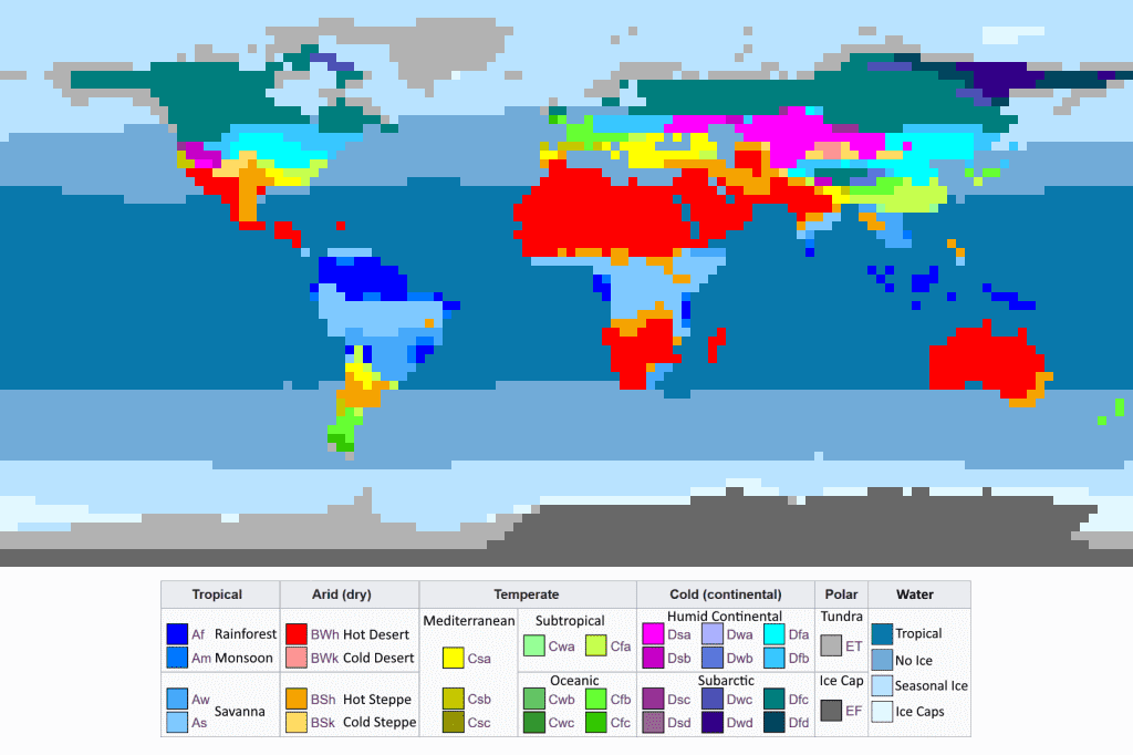
There are a variety of minor differences caused largely by the limited resolutions and variations in ground cover not modeled in ExoPlaSim, but a few major differences stand out:

• Northern Europe is somewhat cooler in the model due to the lack of deep ocean currents.
• Antarctica is partially ice-free and Greenland lacks a major glacier, due to the weaker glacial growth; though they may have got a bit larger had I let this model run longer or started with a colder model and then gradually increased temperatures.
  
• The East Asian monsoon appears to be significantly weaker in the model than reality, making northern China and India drier than they should be in summer and East Africa wetter than it should be. I'm not sure but I think this is somehow caused by the low resolution.
• ExoPlaSim seems to have a bias towards Mediterranean climate patterns (As, Cs, and Ds zones). I'm not really sure why, but averaging the outputs of multiple years together reduces it somewhat.
• Small islands and peninsulas often turn out drier than they should be, which I think is probably a resolution issue again.
  

All that out of the way, let’s get started.

Installation

Firstly, ExoPlaSim is designed to run on a Unix operating system. Per the readme, it should work fine on recent versions of Ubuntu and CentOS (and OpenSUSE, which I’m using). It should also work on Mac OS X, though with a bit of extra work.

For Windows users, there are two approaches to setting up an environment that ExoPlaSim can run on:

• Install a Linux OS of the sort ExoPlaSim was designed for on a partition on your hard drive, such that you can boot to your usual OS or Linux as necessary.
• Install Linux on a virtual machine within your OS.

The first option is probably the best all-round, and it’s the one I’ll be primarily describing today, though I’ll also relay some instructions from some other ExoPlaSim users who’ve gone with the second option.

Installing Linux on a Partition

For this option, you’ll need some extra space on your hard drive you don’t mind setting aside (don’t worry, you can uninstall Linux and reclaim that space later if you need to)—ideally at least 40 Gigabytes, but around 10 GB as an absolute minimum—and an empty USB stick or DVD you can dedicate to the purpose (again, you should be able to reformat it and reclaim it for other uses later).

There are all sorts of different options for Linux operating systems, but per the recommendation of the PlaSim authors I’ve been using OpenSUSE (specifically OpenSUSE Leap 15.3, but any recent or future version should work fine), and I’ll describe it’s use here.

OpenSUSE Leap is available for free on its website in two versions: A larger package which contains all necessary files, and a smaller package which requires connection to the internet during installation, which can be a tad tricky to setup but may be faster otherwise on slow connections (because it doesn’t necessarily require downloading all the software packages). In either case the download will contain a CD image file, and the OpenSUSE website has some instructions on loading this data onto a USB stick or DVD such that they can be used for installing Linux.

Past this point, you won’t have access to an internet browser on your computer until OpenSUSE is fully installed, so you may want to read ahead through the rest of this section and take notes if necessary, or open this page on your phone.

The next step is to insert the USB or DVD, then restart your computer and open the boot manager, which can be done in a few ways, often by pressing the f2, f10, or f11 keys during startup, though this will depend on the model of your computer.

This should open the advanced boot options menu, and you should be able to navigate to a boot manager, where you can both ensure that booting from USB or DVD is enabled and rearrange the boot order such that your computer attempts to boot from your USB stick or DVD before booting up windows from the hard drive. Save these settings and exit, and if everything’s gone right you should eventually come to a menu looking something like this:

For the rest of the installation, you can refer to the detailed guide here. The short version is that you should generally stick with the default options, but there are a couple steps worth highlighting:

• If you’re using the smaller installation package which requires an internet connection, setting up the connection can be, as mentioned, a tad tricky. You should be able to use the same network name and password as usual, but you may have to play around with different settings for connection and security type to find one that works.
  
  
• The “System Role” step determines what your desktop and basic interface will look like. “Desktop with KDE Plasma” is the most similar to Windows, with a taskbar and start menu and so on, and I’ll be assuming its use for the rest of this tutorial.
  
  
• Pay special attention to the next step, “Suggested Partitioning”. This determines how your hard drive will be partitioned, and where OpenSUSE will be installed. For a typical computer with a single hard drive that hasn’t been partitioned before, the suggested setup should be fine; but otherwise, you may want to go through the “Guided Setup” to ensure that the partition is going on the right drive, and no existing operating systems are being removed. You can also alter the size of the partition, though I don’t recommend going much lower than the default 37 GB, as the default software packages add up to around 7 GB, ExoPlaSim will need a bit of space to write files to, and you can always change the partition size later.
  
  
• In the “Installation Settings” step, I suggest keeping the default package. In addition to everything necessary to run a good desktop environment—and ExoPlaSim, when we get there—it includes Mozilla Firefox, an internet browser, LibreOffice, a set of programs analogous to Microsoft Office (LibreOffice Calc seems to run my worldbuilding spreadsheet just fine) and various other tools for viewing and editing common files. If you like, you can sort through the software list and remove more frivolous programs like the games, but those really don’t add up to much drive space.
  
  
• During my installation, I was prompted on installing an experimental graphics driver, and, as per the recommendation, decided against it; so I suppose you can do the same if you get the same prompt.

Once the setup is complete, the installation should take no more than an hour or two. You can restart your computer again, and then from the boot menu choose “Boot from Hard Disk” and select your OpenSUSE partition (in the future, you can rearrange the boot order from your boot manager to allow you to boot into OpenSUSE without the USB or DVD).

Installing Linux on a Virtual Machine

Running Linux on a virtual machine may be a little more straightforward for some people and doesn’t require partitioning your hard drive, though it does require using a command line rather than desktop interface and ExoPlaSim will probably run at least a little bit slower this way.

Friend of the blog Alex (Ostimeus on discord) has been running ExoPlaSim this way using Windows Subsystem for Linux and has provided these instructions, which I’ll also relay here:

First, go to Control Panel → Programs → Turn Windows features on and off. Enable “Virtual Machine Platform” and “Windows Subsystem for Linux”. (if those aren’t available check the installation instructions here).

Restart your computer.

Open the Microsoft Store and use it to install OpenSUSE Leap 15.3. If this doesn’t work the first time, restart, go into the BIOS (the same way I describe accessing the boot manager above) and make sure “virtualization” is enabled. If you can’t get WSL2 working, WSL1 should be fine.

Once OpenSUSE is installed, YaST should open. Use the arrow keys or “Tab” to navigate (all the buttons should also have a highlighted letter, and you can select them by pressing “alt” and that letter”).

Installing ExoPlaSim and Dependencies

Once OpenSUSE is installed and open, and you’ve connected it to the internet (at which point you can open Firefox and return to this tutorial, if you like), you can start getting it set up to run ExoPlaSim. OpenSUSE comes with Python3 installed by default (If you’re using a different operating system, you may need to install it) but we also need some additional packages (essentially, files containing additional functions that python can use) to run ExoPlaSim. But this is pretty straightforward in OpenSUSE:

In the Start menu at the lower left (in the KDE Plasma desktop) go to Applications -> System and open “YaST Software”. For each of the below software packages, type in the name in the search box on the left, find the package in the list that matches that name, press the box to the left of that package such that it shows a “+” sign (if it doesn’t have a check in it already), press “Accept” in the bottom right. YaST will automatically find any dependencies, which you should accept as well, and then install them.

(VM users can open YaST by typing in sudo yast, and then navigate the program using the “Tab” key to cycle between buttons and selection boxes and “Enter” to select them.)

The required packages are:

netcdf

python3-devel

gcc-fortran

gcc-c++

make

openmpi

openmpi-devel

netcdf-devel

(VM users will also need python3-pip)

These next packages used to be necessary for older versions of ExoPlaSim and shouldn’t be required for the current version, but just in case I’ll leave them here for reference:

python3-cairo

libnetcdf_c++-devel

xorg-x11-devel

(I also used to advise getting numpy, scipy, and matplotlib though YaST, but for whatever reason some key files are left missing in the numpy install; fortunately the “pip install exoplasim” step in a little bit will install these on its own, and do so properly, so just let that handle it; to be clear, do not install numpy on its own)

For most of these packages, installing them through YaST is all the setup you need. But the openmpi-devel package (which is necessary for running the model with multiple processors) requires one extra step:

In the Start menu, go to Applications -> System and open “File Manager – Super User Mode”. This allows us to alter files and folders that are usually protected, so you shouldn’t get used to using it, but we’ll need it just this once.

On the bar on the left of the window, you should see a list of “Devices” on the bottom, which will include your partition; it’s labeled as “35.0 GiB Hard Drive” on my installation (you can also access the files in your Windows partition in that list, though this doesn’t always seem to work, likely because Windows includes a “fast boot” function that means it doesn’t completely stop running even when shut down). Within that device, navigate to:

usr / lib64 / mpi / gcc / openmpi / bin

Copy the contents of that folder, and paste them to:

usr / bin

And close the file manager, as we won’t need it anymore; we can use the regular “Dolphin” file manager from here on out. This may not be the most elegant method of getting ExoPlaSim to use these files, but it seems to have worked fine for me.

(VM users should:

• enter cd .. and then ls until it shows a list of files that includes “usr”
• enter sudo cp -r usr/lib64/mpi/gcc/openmpi/bin/* usr/bin/
• if that doesn’t work, you can also try:
  sudo cp -r usr/lib64/mpi/gcc/openmpi/bin usr/bin/bin
  sudo mv usr/bin/bin/* usr/bin/
  sudo rmdir usr/bin/bin
• If this has worked, the number of files within usr/bin should have increased by 68
• make sure to return to the default path using cd)

That done, open “Konsole” (VM users will already by using it); it should be in the favorites tab in the start menu, otherwise look in Applications -> System. This is a command-line interface, and though It may look a little daunting, there are only a few commands we need to input here. One thing to note is that the usual “Ctrl-c” and “Ctrl-v” shortcuts for copy and paste won’t work in Konsole, but right-clicking will still work.

First off, to install ExoPlaSim, type in:

pip install exoplasim[netCDF4] --user

(temporary note; a fair few people have had issues getting version 3.3.0 to work properly, so if that's still the latest release you might want to instead install the previous version with pip install exoplasim[netCDF4]==3.2.4 --user)

It should download and install ExoPlaSim and a couple dependencies (numpy, scipy, and matplotlib, which are also required for some of the scripts I’ll mention later). It may do so haltingly; just wait until it completes and you have a line ending with your username ending in “:~>” before you attempt to type anything more in. It may throw an error about some scripts being outside your “PATH”. To solve this, type in:

PATH=$PATH:/home/user/.local/bin

Where “user” is your username, as shown in the error:

And be sure to run at least one ExoPlaSim script before you next close Konsole; the scripts referred to in the error are only needed for first configuration, but Konsole doesn’t seem to remember the PATH command between sessions. You’ll also need to put this command in again if you ever update ExoPlaSim or alter its files such that it needs to configure again; Alternatively, a more permanent solution would be to open the ".profile" file in your home folder (if you can’t find it, select the icon in the top right of Dolphin and select “Show Hidden Files”), paste in the command and save it. From then on, the command should be run every time you boot up OpenSUSE.

If you ever encounter an error referring to “No module named exoplasim.pyfft’, this indicates that ExoPlaSim was configured without a proper path. The simplest fix is to navigate to home / .local / lib / python3.6 / site-packages (again, show hidden files if you can’t find “.local”), delete “exoplasim”, and then reinstall and reconfigure it.

If all goes well then it’s time to make our first python script to run exoplasim. To open a new script, type in:

kate program.py &

The “program” bit here can be any name, so long as it has the “.py” file type (the “&” bit is also optional, but without it we’d have to close the script to use Konsole again). This should open a new window showing an empty text file (you can also make and edit scripts in the “Home” directory as you would with any text files, I just figured we’d use Konsole while it’s open; and giving the file the “.py” ending from the outset causes the text editor to helpfully color code script elements in a manner appropriate to python, in a similar manner to the embedded script below). You can copy and paste text in here as normal.

(Kate doesn't seem to be installed with the VM version, so VM users should create their scripts in windows using something like notepad++.  You can then open file explorer and type in \\wsl$ in the directory bar, giving you access to the WSL files such that you can drag files in and out.)

First off, let’s run a short script just to check that ExoPlaSim has installed right. Copy this text into your script:

I’ll explain what all this means later, for now the only section you might need to change is the “ncpus” parameter, which indicates the number of processor cores the model will work on. To check how many cores you have, in the Start menu go to Applications -> System and open “Info Center”, which should show your processors under “Hardware”. For example, on my system it shows “Processors: 8

 x Intel® Core^TM i7-7700HQ CPU @ 2.80GHz”, indicating that I have 8 cpu cores, so I’d want to put “8” instead of “4” for the ncpus parameter in my script.

(VM users, if you can find the "Device Manager" in the control panel on Windows, it should include a list of your processors)

Save the script, then return to Konsole, and type in:

python3 program.py

(Or whatever else you called the script, if not “program”.)

The first time you run a model with ExoPlaSim, it will go through a configuration process that shouldn’t take too long. It will spit out a lot of text into Konsole, some of which may be warnings and errors, but so long as there isn’t any red text, you can ignore it all (if there is red text, it probably means you missed one of the software packages). Once that’s done, it will compile the specific model specified in the script and run it. That should look something like this:

You can safely ignore all those “an array temporary was created” warnings, and you’ll know a model year has passed whenever a new batch of them appear. So long as you don’t see something about exoplasim producing junk data and needing to stop, the model should be running fine. To double-check, you can open the “Home” directory (there should be an icon on the desktop, and starting the “Dolphin” file manager will open to it by default) and find a folder called “mymodel_testrun”, within which you should find some files that are being continuously rewritten. There will also be a “snapshots” folder, in which you should find a new file appearing once every simulation year.

(VM users may run into “Permission denied” errors. This may just mean that you need to delete the working directory, e.g. “mymodel_testrun” before running the file again, but if that doesn’t help you may also need to:

• enter cd .. and then ls until it shows you a list of files including “home”
• enter sudo chmod -R a+w+x *home*
• reinstall ExoPlaSim)

Anyway, this test script runs a climate model with all the default settings, at about the minimum reasonable resolution and precision, for 10 years. Depending on your processors, this can take anywhere from under 10 minutes to over an hour—which should give you a rough benchmark of about how quickly your computer will run ExoPlaSim in general. You can do other things like browse the internet while it’s running, though I’m not sure how much that might affect the runtime.

Once it’s complete, ExoPlaSim should show a message in Konsole, delete the “mymodel_testrun” folder, and create a “mymodel_ouput” folder containing the state of the model in the final year of the simulation. If something went wrong it will create a “mymodel_Crashed” folder instead.

Configuring ExoPlaSim

Presuming that everything went well and the model seems to be functioning normally, we can now start creating our own scripts for modeling our own planets. ExoPlaSim has fairly extensive documentation of its own, including some tutorials on running models and interpreting their output, but for the sake of convenience I’ll describe all the parts of the scripting language I think you might need to use for broadly Earthlike planets.

Alex has now made a configuration tool for creating a script (and uploading terrain) via a simple interface, without writing it all up yourself. I still recommend reading through this section to understand what all the options are, and it may be especially helpful if you want to adjust the script or do something more advanced than run a model through once.

To start out with, here’s what a typical ExoPlaSim script might look like (in this case, it’s the setup I’m using for my example world, Teacup Ae; given how many values I tweaked, I strongly recommend using one of the template scripts at the end of this post rather than this one as a basis for your own scripts):

(Note that I’ve added a couple extra lines and spaces here for clarity: in Python scripts, you can add empty lines (though not extra indents), extra spaces before and after operands (=,+,-,*, etc.) and after commas, and use single quotes (‘) or double quotes(“) interchangeably (though any one string must start and end with the same characters, e.g. you can use ‘teacup’ or “teacup” but not ‘teacup”), all without changing the behavior of the script.)

To understand what’s going on and what we can change, lets go through this script line-by-line.

import exoplasim as exo

This just tells python to find ExoPlaSim’s library of special functions, and gives it the shorthand “exo” to refer to them later. You should always include this line at the start of any script for ExoPlaSim.

teacup = exo.Model(workdir=’teacup_run’, modelname=’teacup’,

    outputtype=‘nc’, resolution=’T42’, layers=10,

    ncpus=8,precision=8, crashtolerant=True)

This sets up the model for my planet, and gives it the shorthand “teacup” for referring to it later. Within the parentheses are various parameters for the model. These parameters can be entered in any order so long as they’re all separated by commas (e.g. I could have written crashtolerant=True at the start or in the middle instead, without changing the meaning) and they’re all optional; any parameters you don’t enter will default to values appropriate for a simulation of Earth. Let’s go through the parameters one by one, including a couple I don’t normally use but may be useful to you in the future:

workdir

Sets the path and name of the folder in which the model holds its files while running. As just a name it will put the folder in the home directory, but if you add a path you can place it elsewhere. In either case, paths and names should always be enclosed in single (‘) or double (“) quotes (again, either is fine, but don’t mix them for one name).

modelname

Sets the name used for the output folder and some output files.

outputtype

Controls the filetype of the output files. ‘.nc’ will produce netCDF files, which can be read by a couple of the tools I describe later. Various other types are available, though a few may require additional software packages.

resolution

This sets the resolution used for modelling the planet’s surface, and thus the resolution of the geography we can import into the model and the output we’ll get. These are the resolutions ExoPlaSim can handle, and the associated codes to input here:

Code	T21	T42	T63	T85	T106	T127	T170
Height	32	64	96	128	160	192	256
Width	64	128	192	256	320	384	512

T21 is the default resolution, and you should generally use it for most purposes of testing and playing around, but many details of climate are lost at such low resolution, so it’s best to use at least T42 for outputting actual maps of the planet. Bear in mind that the highest resolution, T170, contains 64 times as many cells as T21, which implies an order of magnitude or two longer runtimes—likely more, as higher resolutions seem to be less stable and so require higher precision modelling in other respects. So far I've only tested T21 and T42 resolutions myself, but I know others who have performed brief T63 runs (~10 model years) on their home computers.

layers

Sets the number of atmospheric layers modeled—in essence, the vertical resolution of the model grid. This is 10 by default, but low-resolution models seem to work fine with 5, which also saves a good deal of computing time. Higher-resolution models may require more layers for best accuracy, but that would even further extend the runtime.

ncpus

As already described, the number of processors to run on, which you should generally set to the total you have available (you can still do other things on the laptop like browsing the internet while the model is using all cores, though it may be a bit slow).

precision

The precision (in bytes) of some internal numbers used, either 4 or 8. 4 will run a tad faster, but may be a little less stable and more prone to crashing, so 8 is the default.

crashtolerant

If set to True, then if the model crashes (and at least 10 years have been simulated), it will rewind 10 years and try again. This can help get around some crashes caused by essentially just random noise in the model, without requiring you to manually restart it each time. On the other hand, if there’s some more fundamental issue with the model (e.g., it’s warming to the point that the oceans start boiling away) then this feature could cause it to be trapped in an infinite loop; so it’s probably best to leave it off if you’re “exploring” new configurations, and to check up on the model when you do turn it on. Note that for this and other True/False configurations, True and False have to be capitalized, and shouldn’t be placed in quotation marks (Kate should helpfully highlight them a different color if you format them right).

inityear

The number to use for the first year of output, with subsequent years counting up from there. May be useful if you’re continuing an old model and want to keep all the years from the full model in order. Do note, though, that the runtobalance command we'll use later requires that you have the outputs from all years from 0 to the current one in your work directory.

recompile

If set to True, forces exoplasim to compile again before running. May be useful if you’ve altered some of the source files (though I won’t discuss anything like that here).

Moving on…

teacup.configure(timestep=40, runsteps=4896,

otherargs={'NSTPW@plasim_namelist':'272'},

flux=0.74*1367, startemp=4500,

year=136, eccentricity=0.1, fixedorbit=True,

rotationperiod=1+5/12, obliquity=30, lonvernaleq=80,

gravity=8.47, radius=0.96,

landmap='t64_surf_0172.sra', topomap='t64_surf_0129.sra',

pN2=1.8, pO2=0.2, pCO2=0.0155,

wetsoil=True, vegetation=2, initgrowth=0.5,

glacier={‘toggle’: True, ‘mindepth’: 2, ‘initialh’: -1})

A couple syntax notes:

• I’ve used the shorthand, teacup, I established in the last line to refer to the model here.
• I’ve broken the parameters inside the function over several lines for clarity; you can break up the parameters any way you want like this, so long as every line after the first is indented by the same amount.
• Any parameter that requires numerical input can also take a mathematical expression. You can use +, -, *, and / as you'd expect, use ** for exponentiation (e.g. 2**3 is 2³), e for scientific notation (e.g. 350e-6 is 350*10^-6), and parentheses for controlling the order of operations.

This line further configures the model (in ways that don’t require it to be recompiled, hence the 2-step configuration). Once again, let’s go through the parameters, this time breaking them down into some broad categories:

Model Setup

timestep

How much time passes in each step of the simulation, in minutes. Longer timesteps will make the simulation run faster, but it may be less stable and accurate. This is 45 by default, but for tidal-locked planets it’s recommended that you reduce it to 30, and in general if you hit a crash—especially if the Konsole output refers to “non-finite temperatures”—your first instinct should be to reduce the timestep. I’ll say a lot more about working with the model’s timekeeping in a bit, for now I’ll just say that it generally seems to work better if there are a whole number of timesteps in a 24-hour day.

snapshots

If set, the program will produce a “snapshot” whenever this number of timesteps passes, recording the state of the model at that particular moment. If using this, it’s recommended to set it to be equal to around 15 days such that it doesn’t slow down the model too much (so, 480 for a 45-minute timestep. 720 for a 30-minute timestep, and so on).

runsteps

The number of timesteps in a simulation year (must be a whole number). By default this is set for a 360-day year, e.g. with a 45-minute timestep it is 11520 (it will automatically adjust to different timesteps if not configured here). This does not alter the simulated planet’s orbital period, or really any aspect of its climate; it merely alters the period of time referred to in later steps that run the model for a period of years, and the length of time represented in the output files. Again, I’ll explain some considerations for the model’s timekeeping a bit later.

physicsfilter

Adds a couple filters to the numbers running through the model, which can help prevent crashes and odd outputs (and in particular removes some artifacts known to arise for tidal-locked planets). For a fairly earthlike planet at T21 resolution, this isn’t necessary, but for tidal-locked planets, planets with very sharp topography, higher resolutions, or any other models that are consistently crashing, it’s recommended you set physicsfilter=‘gp|exp|sp’

restartfile

Path to a restart file. As a model runs, it produces a restart file each year, which holds the current state of the model at the end of that year. If you want to continue running a model after its run (or if you want to try continuing a model that crashed) then you can use this parameter to point the model to that restart file, and it will pick up modelling from that saved climate state. You can even continue running with some of these configure parameters changed (e.g., you can alter CO₂ levels to warm or cool the planet). Note that if you do restart,  you shouldn’t change the resolution, layers, or precision in the exo.model step, but you can probably change everything else (I haven’t tested this thoroughly).

otherargs

Alters an additional internal parameter not usually available through the configure function, in this case NSTPW (I think it’s short for “Number of STeps Per Write”, but I’m not sure) which controls how often data recorded from the model is averaged together. I’ll explain the significance of this later, but for now just know that to change this you only need to alter the number at the end (the 160 in {'NSTPW@plasim_namelist':'160'}).

Star and Orbit

flux

The flux of sunlight hitting the top of the planet’s atmosphere, in watts/meter². By default this is 1367, the value for Earth. Teacup Ae receives 74% as much light as Earth does, hence 0.74*1367. You can determine how much light your planet receives, relative to Earth, with my worldbuilding spreadsheet, or just with the formula [flux] = 1367 * [star luminosity compared to sun] / [distance from star in AU]².

startemp

The effective temperature of the star, in Kelvin, which will be used to adjust atmospheric absorption and surface albedo. It does not affect flux or or year length; the onus is on you to find a set of values corresponding to a realistic scenario (if you want to). If not set, a sunlike star will be assumed.

year

Length of the year, in 24-hour Earth days. Defaults to 365.25, the value for Earth. This controls the period the planet takes to orbit its star, not the length of the years used for the output files and the model run controls—those are set by the runsteps parameter, though generally speaking you should probably make them the same, except for very short orbital periods. Again, you can use my worldbuilding spreadsheet to help determine this and other values—or you can use [orbital period in years] = sqrt( [semimajor axis in AU]³ / [mass of star compared to sun].

eccenticity

Eccentricity of the planet’s orbit. Defaults to 0.016715, the value for Earth.

fixedobit

True forces the orbit to remain unchanged throughout the simulation, False allows for ExoPlaSim to calculate Milankovitch cycles to alter the planet’s orbit and orientation. The latter feature is still under development, so it’s probably best to keep this on for now.

Rotation

rotationperiod

Rotation period of the planet, compared to Earth. This is a sidereal day (23 hours 56 minutes for Earth), but for planets with many orbits per year it should be an insignificant difference from a solar day, so don’t worry too much about the difference. Defaults to 1.

obliquity

Obliquity, A.K.A. axial tilt, in degrees. Defaults to 23.441, the value for Earth.

lonvernaleq

Longitude (angle along the orbit) of periapsis (point when the planet is closest to the star) in degrees, measured from the autumnal equinox, which is used to orient the planet’s rotational axis relative to its orbit. Defaults to 102.7, the value for Earth. This should be 90 degrees less than the argument of obliquity (adding 360 if the result is below 0), so:

0: periapsis coincides with the autumn equinox in the northern hemisphere

90: periapsis coincides with the northern winter solstice

180: periapsis coincides with the northern spring equinox

270: periapsis coincides with the northern summer solstice

(Okay, formally “longitude” is a compound angle measured along two planes, but if we consider the orbit to have 0 inclination, then those become the same plane and match the orbital plane. Also, most sources will say that longitude of periapsis is measured from the vernal equinox, but what they mean is that it’s the point on the object’s orbit that’s directly overhead during midday on the vernal equinox, and if you’re measuring this for the body you’re standing on, it’s actually the point on the opposite side of the orbit; hence, the autumnal equinox.)

Tidal-Locked Planets

A couple of parameters specifically for use with planets tidally locked into a 1:1 spin-orbit resonance. Because of small errors in the model’s internal timekeeping, we can’t simply match the rotation period and year length; the errors will cause the substellar point to drift over time. Instead, tidal-locking is modelled by locking the substellar point to a given latitude. This means that the substellar point can oscillate north and south for planets with nonzero obliquity, but currently it won’t oscillate east and west as it should for planets with eccentricity. This should be fixed in the future when proper orbital simulation is added to ExoPlaSim, which will also allow for easier simulation of other spin-orbit resonances.

synchronous

True locks the sun to one longitude.

substellarlon

Longitude of the substellar point, in degrees. Defaults to 180; though if you import geography by the method described later, starting with a map with 0 longitude at the center, then the geography of your map will be offset 180 degrees from the model’s coordinate system, so the default of 180 would actually place the substellar point at 0 longitude (you may want to run a quick test when setting up a model like this to ensure everything’s in the right place).

desync

Rate at which the substellar point drifts from its initial longitude, in degrees per minute (I presume to the east). You could use this to approximate spin-orbit resonances other than 1:1 (i.e. drift of 180 degrees per orbit would approximate the 3:2 resonance), but again the effects of eccentricity on the movement of the substellar point are not properly modelled in the current version of ExoPlaSim. Defaults to 0, can be positive or negative.

tlcontrast

Adds an initial temperature contrast between the substellar point and the antistellar point, in Kelvin. Defaults to 0. Increasing it to, say, 100 might help the model balance faster.

Planet

gravity

Acceleration due to gravity at the planet’s surface, in meters/second². Defaults to 9.80665, the value for Earth.

radius

Radius of the planet relative to Earth.

landmap

Path to a .sra file containing a land/sea mask for the planet’s geography. We’ll discuss how to make these files later. If you don’t define a landmap or topomap, it’ll default to Earth’s geography (at least for T21 and T42 runs).

topomap

Path to a .sra file containing the planet’s topography. Again, we’ll discuss how to make them later.

orography

Scaling factor applied to the above-defined topography, down to flat continents at 0.0. Extreme conditions on high mountain peaks or deep valley floors can sometimes cause crashes, so flattening out the topography can help you tell if that’s the issue.

aquaplanet

True erases all land surfaces (including the default earth geography) and gives you a uniform, all-ocean planet. This may run a bit faster, so it can be useful for debugging or quick tests of other factors.

desertplanet

True erases all seas and gives a fully land-covered planet.

Atmosphere

Can be set in two ways:

• Set the partial pressures of all the gasses in the atmosphere, out of the list of preset gasses, and allow ExoPlaSim to calculate total surface pressure and the effective gas constant.
• Set the total surface pressure and gas constant directly, and optionally set the partial pressure of some of these gasses out of that total.

Be aware that the model can struggle a bit with surface pressures greater than 10 bar or less than 0.1 bar; it can be done, but you may need to significantly reduce the timestep, to as little as 5 minutes. Also bear in mind that some of the model’s internal workings assume an atmosphere with broadly Earthlike composition (nitrogen/oxygen dominated), and so may not be fully accurate for other atmospheres.

pH2

Partial pressure of hydrogen (H₂) in bars.

pHe

Partial pressure of helium (He) in bars.

pN2

Partial pressure of nitrogen (N₂) in bars. Earth has 0.7809.

pO2

Partial pressure of oxygen (O₂) in bars. Earth as 0.2095.

ozone

True adds an ozone layer, which slightly increases greenhouse heating, among other effects. Any planet with oxygen should probably have some ozone as well, but ExoPlaSim’s handling of ozone has been tuned to match Earth and may not be very accurate for significantly different atmospheres or stars. At a guess, I’d say you could maybe still use it for Earthlike planets with significant atmospheric oxygen orbiting sunlike stars, but it may be best to exclude otherwise, even though this may cause a slight underestimate in greenhouse heating (though that’s already the case for planets with high CO₂).

pAr

Partial pressure of argon (Ar) in bars. Earth has 0.0093

pNe

Partial pressure of neon (Ne) in bars.

pKr

Partial pressure of Krypton (Kr) in bars

pCO2

Partial pressure of carbon dioxide (CO₂) in bars. Other than ozone, this is the only greenhouse gas you can directly set. Earth had around 0.00028 prior to the industrial revolution, and at time of writing is rising past 0.000416, but the model defaults to 0.0003.

pH2O

Partial pressure of water (H₂O) in bars. This only affects surface pressure and the gas constant; it is not referenced in determining humidity, any aspect of the water cycle, or greenhouse heating by water vapor.

pressure

Total surface pressure in bars. Unnecessary if you’ve already set all the partial pressures of the component gasses in your atmosphere, though you can combine this with the partial pressures of some of the component gasses (in which case you should set a gas constant as well). Defaults to 1, if no partial pressures have been set.

gascon

Effective gas constant, in Joules / (kilograms * Kelvin). Can be calculated as the molar gas constant (8.314 J / K*mol) divided by the average molar mass of the atmosphere, in kg/mol. Defaults to 287, the value for Earth, if no partial pressures have been set.

Surface

wetsoil

True alters the albedo of land surfaces based on how wet they are; wetter land has a lower albedo, so it reflects less light.

soilalbedo

Can be set to a fixed albedo value that will be used for all land. You usually shouldn’t do this for Earthlike planets, but you can use it to model some sort of unusual desert planet covered in more reflective desert sand or salt.

vegetation

Controls a vegetation model, which will impact surface albedo and humidity. It’s not a very advanced model and probably won’t handle particularly exotic climates too well, but it’s still nice to have. 0 or False will leave the model off, 1 or True will activate "diagnostic" vegetation which is fixed to an initial value of vegetation cover across all land, 2 will activate a coupled vegetation model which will grow and die back in response to the local climate, and produce an estimate of the resulting forest cover in the output. This will probably slow down the model to some extent, so you might want to leave it off until you’re putting together a final model.

vegaccel

Accelerates the rate of vegetation growth. 1 by default, must be an integer. I don’t know of a specific case where you’d want to change this, but it’s there if you need it.

initgrowth

Adds vegetation cover to all land at the start of the model, which might save some time running the model to equilibrium and make the resulting climate somewhat less arid than it would be if it started without vegetation. Should be between 0 and 1, 0.5 is probably good for most cases.

glaciers

Controls the formation of glaciers. As it stands, turning this on allows for persistent deep snow in a cell to form glaciers, but these glaciers don’t flow outward into other cells as would be realistic, so this model may underestimate the extent of large continental glaciers. It’s a sort of compound parameter with a different syntax:

glaciers = {‘toggle’: True, ‘mindepth’: 2, ‘initialh’:-1}

Going through each subparameter:

toggle

True allows for new glaciers to form. False by default.

mindepth

Sets the minimum depth of accumulated snow required for glaciers to form, in meters. 2 by default.

initialh

A value of 0 or greater will place glaciers with that depth in meters over all land surfaces when the model starts, and a value of -1 will not add any initial glaciers.

That’s about wraps it up for the configure function, though there are some additional options I’ll discuss later.

teacup.cfgpostprocessor(times = 12)

This configures the postprocessor that converts the model’s data into readable output files. Here I’m just using the times parameter to set the number of months per year in the output (it should be 12 by default, so it is actually redundant here).

teacup.exportcfg()

This line saves all that configuration information (from the teacup.configure line, not from exo.model line) into a config, by default named with the set modelname. Then you can run the same model later by just loading that config, e.g. teacup.loadconfig(‘teacup.cfg’)

teacup.runtobalance(baseline=10, maxyears=100, minyears=10, timelimit=480,

          crashifbroken=True, clean=True)

This is the main command to run the simulation. We used a simpler run command before where we just specified the number of years, e.g. teacup.run(years=100). But this runtobalance command instead runs the model until it appears to have reached equilibrium, as judged by the balance between average incoming sunlight and outgoing heat remaining unchanged over several years. How long this takes can vary quite a bit, so it helps to have this option rather than having to guess a reasonable timeframe. Anyway, here are the parameters:

baseline

How many years the simulation has to remain at equilibrium before it is determined to be at balance (i.e., the amount of drift per year in the balance of incoming and outgoing energy has to remain below the threshold for this many years). Defaults to 50, but for our purposes around 10 Earth years is usually fine.

maxyears

The maximum number of years for the simulation to run, even if it hasn’t reached balance by the end. Defaults to 300.

minyears

The minimum number of years for the simulation to run, even if it has reached balance by the end. Defaults to 75, but again a low number like 10 is usually fine, and can especially save time at higher resolutions.

timelimit

A time limit in minutes for the simulation. If set, the model will dynamically alter the maxyears parameter to attempt to end the simulation before this limit.

crashifbroken

This just helps make crashes a little more graceful and gives you somewhat more useful error reports.

clean

Deletes temporary files produced each year once an output has been created, which should help limit the amount of hard drive space used while running.

teacup.finalize()

Moves the output files to a new folder, named according to the first parameter (‘teacup_out’ here; this must be placed first in this case)

allyears

If set to True, moves the output files from every year of the model run; otherwise, it only moves the final year. These output files can take up a good bit of hard drive space, but if you’re making a final run you intend to use for a Koppen zones, I suggest using this so you can average together the data from multiple years when making the map. False by default.

keeprestarts

If set to True, moves the restart files—which can be used to restart and continue running the model—as well as the outputs. False by default.

clean

If set to True, deletes the model run folder and all files after making the new folder. True by default.

teacup.save()

This saves the model in its current state as a numpy file. By default it will be saved as a .npy file with your model name, but you can also enter a name inside the parentheses (in quotation marks). You can then load it again in another script like so:

import exoplasim

import numpy

numpy.load(‘teacup.npy’).item()

Unlike a restart file, this doesn’t require any other setup commands and will remember the year of the model and information from previous years; in essence, it allows you to pick back up from the same point in the script as when you saved it. However, it requires the other files in your model's run folder, including outputs from all years for the runtobalance function, whereas a restart file is self-contained (within your computer, anyway; a restart file moved between computers is unlikely to work properly); so using restart files can help save a lot of hard drive space.

Regarding Timekeeping

Though I’ve mentioned some of the constraints of specific parameters related to how the model keeps time, let’s take a moment to put it all together.

See, the ultimate goal here is to produce a Koppen climate map, but the Koppen scheme wasn’t really built with exoplanets in mind. On earth, Koppen zones are defined by monthly averages of temperature and precipitation (1/12 of the year), as well as total precipitation over summer and winter (1/2 of the year) and whether temperatures over 10 °C last at least 4 months (1/3 of the year). So if we want a Koppen map for a planet with a year, say, half as long as Earth’s, we have to ask: is it better to ensure the year is still divided into as many months as Earth (12 months of ~15 days each) or is it better the ensure that each month is as long as on Earth (6 months of ~30 days each) to ensure that the map is accurately reflecting how different seasonal patterns affect local climate and life? And if the latter, what do we do when the number of ~30 day months in a year can’t so easily be split into halves and thirds?

We also have to consider whether our paradigm of seasons can reasonably be applied to very short-period planets, even those with significant obliquity or eccentricity. If a year is only 10 days long, are trees going to shed their leaves in fall just to regrow them in spring 5 days later? Reasonably, there must be a point where annual climate variations go from “season-like” to “day-like” in terms of their impact on life, but where would it be?

I can’t say I know the right answers to these questions, but ExoPlaSim functions in such a way that it constrains our options somewhat. Here’s a basic summary of how the model handles its timekeeping:

The model runs in steps, and the interval between them is set by the timestep parameter. Each step, it saves some data about the current state of the planet to memory. If you have set the snapshots parameter to some value, then at regular intervals (that number of timesteps) the data from the current step will be saved to a dedicated file (and all snapshots are ultimately saved to one file for the year).

But we’re mostly concerned with the main output. After a certain number of timesteps have passed, determined by the NSTPW parameter, the recorded data will be averaged together, and those averages will be saved to memory. This helps limit the total amount of memory the model has to use at once.

After a larger number of timesteps, set by the runsteps parameter, the model will save its recorded data to file. This is done by taking the averaged data recorded at each NSTPW interval, dividing these up based on the number of desired months—set by the times parameter—and then averaging the data in each month, to get one averaged value for the whole month for each data parameter. The result is output as a netCDF file (if you’ve set that filetype). If we want to produce Koppen climate maps from these output files, then each file should represent a year—one complete orbit of the planet around the sun, which is determined by the year parameter.

Ideally, we want an even number of NSTPW intervals in each month, so that each month in the output is representing an even amount of time in the simulation (the model will attempt to interpolate data if there are uneven numbers of these outputs in each month, but we should still try to avoid that necessity). Thus, if we have 12 months in a year, there should be some multiple of 12 NSTPW intervals in a year (in mathematical terms, we should ensure that NSTPW = runsteps / (times * n), where n is an integer). However, by default NSTPW is calculated from the timestep such that it’s interval is about 5 days (120 hours), and we shouldn’t move it far from this value; a much shorter interval would require the model to average together and write out data more frequently, which will slow it down, whereas a longer interval will increase the amount of memory the model has to use, which can cause it to crash.

We also ideally want an even number of days each month—in terms of solar days, set by the rotationperiod parameter (sort of; strictly it alters the sidereal day, and I'm not totally clear on whether ExoPlaSim uses the year parameter to determine synodic days, but for large year/day ratios it shouldn't matter much), not 24-hour Earth days—or else we might get some odd edge effects (e.g. one month may get more daytime hours and the next more nighttime hours, such that the former has a higher average temperature even if daily average temperature is constant).

Thus, here are the overall meanings and limitations of these values (in the associated expressions, n must be an integer, though not necessarily the same integer in each case):

• timestep: the length of each model step, in minutes. Generally the model seems to work best if there is an even number of timesteps in a 24-hour Earth day; so timesteps of 5, 6, 10, 12, 15, 18, 20, 24, 30, 36, 40, 45, and 60 minutes are all decent options.
• (24 * 60) / timestep = n
• NSTPW: how often data is averaged together, in number of timesteps. The amount of time this represents should be kept close to 120 hours. It need not necessarily be a whole number of solar days, though that may be convenient to help keep things straight.
•  ~4 < (NSTPW * timestep) / 1440 < ~6
• runsteps: how often averaged data is written to an output file, in number of timesteps. We’re taking this to be a “model year”, though it doesn’t directly control any aspect of the planet’s simulated orbit. Should contain a whole number of NSTPW intervals.
• runsteps / NSTPW = n
• year: the length of the planet’s orbit, in 24-hour Earth days. To properly produce Koppen maps from the output files, this should be the same length of time as the model year.
• year * 1440 = runsteps * timestep
• times: the number of output times in the output file for each model year, taken here to represent “months”. Per our earlier discussion, for use with the Koppen system, you may want to keep this as 12, or at least some multiple of 6. Each month should contain an even number of NSTPW intervals.
• runsteps / times = NSTPW * n
• times = 6 * n
• rotationperiod: the length of a solar day (roughly), in 24-hour Earth days. Ideally there should be a whole number of timesteps in a solar day, and a whole number of solar days in a month.
• (rotationperiod * 1440) / timestep = n
• runsteps / times = (rotationperiod * 1440 / timestep) * n

This can be a lot to handle, and it’s not strictly necessary that all of these be true; again, the model can interpolate data some if the NSTPW and month times don’t quite line up right. But you should try to tweak you parameters somewhat to accommodate the model’s limitations where you can.

So, let’s consider Teacup Ae’s case: we’ve established previously that the planet has 34-hour days, and 93 of those days in a year. But for purposes of the model we can round that up to 96 days (136 Earth days), so it can be divided into 12 months of 8 days each. Each month will be 272 hours long, 11 1/3 Earth days. We can thus slightly increase the NSTPW interval from 120 to 136 hours (5 2/3 Earth days) for 2 writes a month. 136 hours unfortunately doesn’t divide evenly into 45-minute timesteps, but it should work with 30-minute, 40-minute, and 60-minute timesteps, with corresponding write intervals of 272, 204, and 136 timesteps. And we can adjust runsteps accordingly for a 3,264-hour year, and set the year parameter to 136 Earth days.

As a final note, there is still the aforementioned case where orbits are so short that the planet doesn’t really have “seasons” in the sense we understand them. 24 Earth days is about the minimum year length for which we could reasonably interpret Koppen zones from the model output (4-day NSTPW interval * 6 months), but really I’d be skeptical applying it to anything with a year shorter than a couple months (~60 days). In these cases, it may be best to apply a reduced set of “seasonless” Koppen zones, as I’ve done in the past. Model years should then contain multiple orbits (ideally a whole number of them), such that we’re working with data over a broader length of time and we’re not filling up hard drive space with tons of output files. There’s no particular restriction on how many months to include per year in this case, but we should still probably have at least 1 per orbit, and an even number of NSTPW intervals per month.

Importing Topography

ExoPlaSim reads topography from a pair of .sra files: one is a binary land/sea mask, indicating which cells are to be read as land surface, and which are sea; and the other contains elevation data in the form of “geopotential height”, which is just the elevation in meters multiplied by the acceleration of gravity in meters/second². The .sra files are just strings of data values, but inputting them manually each time would get pretty tedious. Fortunately, friend of the blog Alex (again) has put together a script that can convert greyscale heightmaps to .sra files.

To use this function, first prepare a greyscale heightmap of your world, with whiter areas representing higher elevation, on a linear scale. If you’re using paint.net (though that’s only available on Windows, so you’d have to switch between operating systems), you can expand the colors window, go to the “HSV” section on the lower right, set the “S” slider to “0”, and use the “V” slider to set elevation: so for example, you could draw in the oceans as “0” (completely black), draw in your highest peaks as “100” (completely white), and then somewhere at half the elevation of your highest peaks as “50”.

(GIMP, which can run on linux, should have similar functionality, but the scripts we'll use in a bit don't seem to like to take image files produced by GIMP as inputs, for reasons I haven't quite pinned down).

It’s not vital that you use the full range, though; you could set your highest peak at “80” and your oceans at “20”, for example—though you’ll need to know the greyscale value of your oceans later, so it’s probably best to keep them at “0” for the most part with the land surface scaling linearly from 0 to its maximum value. And there’s no need to mark out underwater bathymetry—it may even cause issues with the climate model—so just use a flat ocean surface. Here’s what the result looks like for Teacup Ae:

We'll explore how to construct more detailed greyscale heightmaps in a later post, but for now such a rough sketch will do fine for the low resolution of the climate model.

Next, make sure the whole map is sized properly. The map should be in an equirectangular projection—with a 2:1 width:height ratio, and all lines of latitude and longitude equally spaced—and it should be an even multiple of its target resolution in pixels. So, for example, if you want to use the T21 resolution in exoplasim, which is 32 cells tall by 64 wide, then you’ll have to use an image that is some multiple of 32 pixels tall, and twice as many pixels wide. The above image, for example, is 512 pixels tall by 1,024 pixels wide.

Save the image (any common filetype should do, I’m using .png).

To convert the image to sra files, you can use Alex's tool, and conveniently make your script at the same time (you can also reuse the same sra files between scripts for the same terrain). If you do so, you can skip the rest of this section.

There's also a standalone python script you can use in your linux partition. As this post was written before the above tool was available, I've written a whole tutorial for it. I no longer recommend this approach (in particular, it won't include any later bugfixes bundled in the above tool), but I'll leave the tutorial in place for now:

Go into your linux partition and download the script Image2sra2.0.3.py, which can be found here (alongside a couple others I'll discuss later). Place it in your “Home” directory alongside the heightmap image, and then open Konsole and type in:

python3 Image2sra2.0.3.py

(or whatever version of the script you have, should it be updated in the future.)

You’ll then receive a few prompts in the konsole window. Most are self-explanatory, but just to be sure we’re on the same page:

First, you’ll need to input the path of your heightmap file; if the file is in the “Home” directory alongside the script, you can just use its name (you don't need to place it in quotes or anything, but do include the filetype suffix). The script will then say if it found the file; if not, try again.

Next, you’ll be prompted on whether or not to include any oceans in the land/sea mask; if you input n, the script will fill in all cells as “land”, regardless of elevation—this would be appropriate for all-land planets. Otherwise, you’ll then be prompted on the level of your oceans on your heightmap on a 0 to 255 scale of brightness; if you marked them black as recommended, this should just be 0.

Next, you’ll have to input your highest elevation in meters, measured relative to the lowest elevation on the map. The image is scaled vertically before the resolution is reduced, so input the highest elevation on your heightmap even if it only occupies a single pixel.

Next, you’ll have to put in the acceleration of gravity on your planet in meters/second². This should be the same as in your model configuration (if you intend to test different levels of gravity for a planet, you'll either have to make new .sra files or use the orography parameter to alter topography by the inverse of the you're altering gravity by).

Next, you’ll be prompted on a debug option: if you select y, when the script completes it will output images showing the areas marked as land or sea at both the resolution of the input image, and that of the output files; this helps to check if there were any issues with how the script interpreted your image. Note that, while this script will mark partial land cover (e.g. a cell with 60% land cover will be marked as 0.6) and ExoPlaSim accepts data in that form, it appears that the data is internally treated as binary: cells below 0.5 land cover will be modeled as fully ocean, and others as fully land.

The script will then spend a little time interpreting your heightmap, and when done prompt you on the “latitude resolution”. This is the height of the climate model resolution; so for T21 it will be 32, for T42 it will be 64, etc.

If your image has the proper resolution to allow for this, the script will then spend a little time downsampling your image, and then finally ask you to give a name for the output files.

It will then output a pair of properly formatted .sra files in its directory; the file ending in 0129.sra contains your topography data, and the one ending in 0172.sra contains the land/sea mask. You can use the topomap and landmap parameters in the configure command of your model script to input these into the model.

Interpreting the Output

There are a few different ways to look at the output of the model, and if you’re not afraid of learning some code then you may want to look into using the included matplotlib functionality. For the rest of us, though, we can look at the data in the netCDF output files using Panoply, which you can download here.

Unzip and place the folder wherever convenient, click the "panoply.sh” file, and choose the option to “execute” (if you don’t get the option and it just opens as a text file, right-click on it, select “properties”, go to the “Permissions” tab and check “Is executable”, then try again). That should open a screen like this (you may have to give it a minute):

You can navigate to a netCDF file you want to look at, and select “Open”. This will bring up a list of output variables. There are a lot here, most meaningful only to climatologists, but you’ll probably be most interested in:

• cl: cloud area fraction in layer: the fraction of each cell covered in clouds at each atmospheric layer, on average
• clt: cloud area fraction: the total cloud area fraction across all layers.
• czen: cosine solar zenith angle: a representation of how high the sun is at midday; acos(czen) will give it to you in degrees.
• glac: glacier cover
• grnz: ground geopotential: the model topography, to use as a reference.
• maxt: maximum temperature
• mint: minimum temperature
• pr: total precipitation
• prsn: snowfall
• ps: surface air pressure
• sic: sea ice cover: as a fraction of area
• sit: sea ice thickness
• snd: surface snow thickness
• wnd: wind speed
• ta: air temperature: in the atmosphere, broken down by each atmospheric layer
• tas: air temperature 2m: the air temperature at 2 meters above the surface, which I’ll use later for determining climate zones on land.
• ts: surface temperature: I'll use this for determining sea climate zones.
  
• vegf: forest cover
• vegnpp: forest net primary production: this is the total mass of carbon converted from CO2 to organic compounds by photosynthesis and not ultimately consumed by the plants themselves. As I'll explain in later posts, this is a decent measure for roughly how much life a region can support and how much food it can produce.
  

Select a variable, press “Create Plot” at the top left, and accept the default longitude-latitude color contour plot, and it will produce a plot of that over your world’s surface (there will be a map of Earth overlayed by default, but you can turn that off in the “Overlays” tab, and go to “Edit” → “Preferences” to stop it turning on by default).

 

In the “Array(s)” tab you’ll see options for which month to display data from (it’ll show a specific timestep in that month, but the data has been averaged for the whole month). For some variables it’ll also show atmospheric layers; the highest-numbered layer (e.g., layer 10 if your model had 10 layers) will be the one closest to the ground (the "sigma" value associated with each layer is the atmospheric pressure at the layer's center relative to the surface air pressure in that cell). If you switch layers and the plot is mostly one color, pressing “Fit to Data” should fix it. In the “Array(s)” tab you can also choose whether to interpolate the data—smoothing it between the cells in the ExoPlaSim model grid—or just show the raw data.

There are numerous options in Panoply for displaying data in different ways. To name just a few options:

• The “Scale” tab includes various options for different color scales to use for the plot, and allows you to adjust the endpoints of the scale and the map key.
  
  
• The “Grid” tab allows you to alter the map projection. I’ll discuss map projections at length in a later post, but a couple good options are “Equirectangular”, which can be projected onto a globe in programs like GPlates and MapToGlobe; “Mollweide”, a popular equal-area projection that I’ve used in the past; and “Winkel-Tripel”, a popular compromise projection. You can also adjust the central longitude; if you want it to look the same as your original topography map, set this to 180 °E.
  
  
• The "Overlays" tab can be used to overlay transparent images on these maps, such as coastlines. Use "File" > "Open" to select such an image and then you can place it as an overlay, like so (note that you may have to offset the image first by 180°, and that you could probably get a cleaner appearance with a shapefile produced from a vector program, rather than the one I did here quickly in paint.net):
  
  
  
  
  
• In addition to the longitude-latitude plot, you can also produce a plot of zonal averages (showing the average for some variable across latitude) and use a line plot to chart the variable for one location (or a zonal average again) across the year.
  
  
  
  
  
• You can also combine plots, which is useful for mapping out wind. First make a plot of ua, eastward wind, and then select va, northward wind, and press “Combine Plot” and select the existing ua plot. In the “Array(s)” tab, select “Vector Magnitude” for your plot. The plot will now be populated with arrows showing the wind direction across the surface, with the color shading now showing the wind speed. You can tweak with the reference value in the “Vectors” tab to adjust their size.
  
  
  
  
  
• Finally, you can export these images, either alone, or together as an animation with “File” → “Export Animation…”, either as an MP4 video or a series of images that you can stitch together into a gif using tools like ezgif.
  
  
  
  
  

I've also now put together a small script to average together multiple netCDF files and also produce a file of annual average values, which you can find as "eps_avg.py" here (same repository as the Koppen zone script I'll discuss in a moment). This file requires NCO to run; find nco in YaST and download it with all dependencies, and then in konsole type in:

pip install nco

Much as with the other scripts discussed, you can run it with:

python3 eps_avg.py

It will then display a few prompts which I'll quickly run over:

• First, it will ask you to input netCDF files: you can either point it directly to a file or a folder, in which case it will find all files inside it with the .nc type (so only do this with a folder containing the last few years you want averaged together, not the whole model run). It will keep prompting you until you type in stop. You can just input a single file if you want to use the other features here rather than averaging together multiple files.
• Next, it will ask if you want to offset months, allowing you to shift forward or back what month the file starts on. The Image2sra script tends to create models that effectively start in November (i.e. around 2/12 of the year before winter solstice) so for a 12-month output an offset of 2 will shift the file to start in January. You can also offset back with negative numbers, so long as the magnitude of offset is not more than a full year. Otherwise just put in 0 for no offset.
• Next, it will ask if you want to rotate latitudes. This will convert the file's longitudes from the [0, 360) range ExoPlaSim outputs to a [-180,180) range with the new 0 longitude where the 180 longitude used to be. This will make the Panoply maps properly centered (so you don't have to use offset overlays).
• Next, it will ask if you want to produce annual averages as well. This will produce an additional netCDF file with the same averaged data, but now all averaged to single annual averages; so rather than monthly averages for temperature, precipitation, etc, there will be a single average over all months.
• Finally, it will ask you to give a name for the output; the annual average will have "_ann_av" appended.

The Koppen Zone Script

This is a script I wrote in Python to read the netCDF files output from ExoPlaSim and interpret the climate data within them to produce maps of Koppen climate zones for your world. You can find it here. In addition to python, it depends on the netCDF4, numpy, scipy, and PIL packages (all of which should already be installed if you’ve been following the tutorial). You modify and share this script if you like, but please link back to worldbuildingpasta.blogspot.com and indicate any changes.

·       I’ll explain the use of defaultcolor.ini; for now, it’s not necessary for basic use of the script.

Though the script is intended to be rather straightforward, there are a number of options and features that may require more explanation.

Let’s start with the most basic use. For convenience, place koppenpasta.py and the NetCDF file you wish it to interpret together in the “Home” directory. In Konsole, type:

python3 koppenpasta.py

Once it starts, it’ll prompt you to input the path to your input file:

If they’re in the same directory, as recommended, you can just input its name (including .nc).

As of version 1.1, you can now also enter a directory (i.e. the name of a folder) and the script will find every file with the ".nc" type in that folder and take them as inputs, reporting their names in konsole as it finds them. So, for example, if you have a folder called "myModel" containing the last 10 years of output for your model, typing in myModel will load up all those files. I'll explain how the script handles multiple input files shortly.

If it finds the file, it will then prompt you on the advanced setup:

For now, respond n to skip.

The script will then run, loading data from the input file, interpreting it, and drawing it out to an image file, named “output.png” by default. It'll then ask if you want to run again with different configuration options, but again you can respond n for now

Once the script reports completion, you should be able to find that file in the same directory as the script. It should look something like this (you may have to zoom in a bit when you open it):

This is a map of your world’s climate zones at the same resolution as the climate model (in an equirectangular projection). A bit blocky, but that’s the limitation of the model.

Now that we’ve got that down, let’s go back to see what options become available if you answer y to the “Advanced setup” prompt. Each of these is accompanied by a short explanation in Konsole, but I’ll describe their function and intended use in a little more detail here. Most of these prompts are numbered lists, with each number keyed to an option such that you can select an option by inputting the corresponding number. 0 is always the default option (and all the (y/n) prompts will also interpret 0 as “no”, for convenience).

Allows you to add more netCDF files as input. If you answer y you can specify more input files, just as you specified the first. Enter as many as you like, and then type stop to indicate there are no more files (for now, this doesn't work with directories like the first prompt does).

The script will then average the data from all these files together, such that for each cell of the climate model, it finds the average climate for each month of the year across that period, and then uses that for determining climate zones. A map produced from one year’s data is fine to get a quick sense of climate, but averaging together data like this gives a better picture of long-term climate and ensures the output isn’t biased by one year’s random variation (e.g. an otherwise wet area that happened to have a drought in the last year of the simulation might be marked as arid if you were using data from only that year) so I recommend doing this for any final outputs.

To work properly, you should put in only files from the same model run that share the same topography, resolution, and number of months. To make sure all your input are from after reaching equilibrium, you should also try to use as many years as the baseline in your runtobalance command (e.g. if you use a baseline of 10, only use the last 10 years of the model output)—though you could also restart the model and run it further with the same parameters to produce more output for increased accuracy.

I’ll explain saving and loading configs later.

Determines the set of climate zones to use on land. By default the script finds the whole set of 31 climate zones, like so:

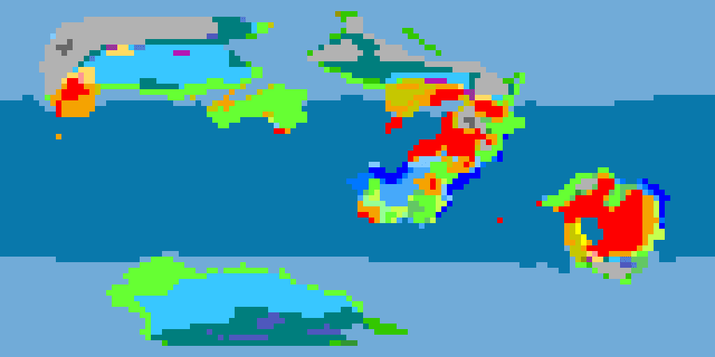
But you can also exclude the Aw/As distinction (as many sources do);

Find only the reduced set of 14 zones used in Part VIb and many other worldbuilding tutorials;

Find “seasonless” zones—in this case, the script will average data from all months together and find climate zones using only that averaged data, marking out only the 9 Koppen zones that are possible without seasonal variation;

I've also used seasonless seas here, but you can choose the behavior for land and sea climate zones independently. Naturally this wouldn't actually be sensible to do with this model of Teacup Ae.

Or just mark out the 5 Koppen groups:

The reduced sets may be easier to read for people less familiar with the Koppen system, and also make for easier comparisons between different climate scenarios. The seasonless zones are appropriate for worlds with no obliquity or eccentricity, or very short orbits.

Finally, there is an experimental option to mark out an approximation of Holdridge Life Zones. This is an alternative climate zone scheme that doesn’t depend so much on seasonal variations.

Typically these are defined by 3 parameters: total annual precipitation (don’t worry, the script will account for different year lengths), annual average biotemperature (average of temperature except that any temperatures below 0 °C are counted as 0 °C, and those above 30 °C are counted as 30 °C), and potential evapotranspiration (the maximum amount of water that could evaporate or be transpired by plant life, were there limitless water in the soil).

However, there’s a lot of variation in exactly how exactly these parameters are used to define the zones with no single standard, and ultimately you can approximate the system using just 2 of them, though you will lose some detail in the boundaries between zones. Potential evapotranspiration is pretty difficult to approximate, so for the moment I’m only using precipitation and biotemperature, following the rough boundaries in this popular figure (and using the same colors):

Because I'm only using biotemperature and precipitation, the zones should actually appear as parallelograms on this chart, not hexagons. Peter Halasz, Wikimedia

Also note that:

• For Holdridge zones there is no particular requirement for the number of months in the files read, and indeed the measurement of biotemperature will be more accurate the more data points it has to read from (i.e., more months).
• The definition of biotemperature presumes that photosynthesis is usually only active between 0 and 30 °C, which may not be accurate for alien life.

Determines the set of climate zones to use in the oceans. By default the script uses the sea zones I defined in Part VIb (though in this case using the sea ice data from ExoPlaSim rather than guessing the extent of sea ice from temperature) but as with land zones, there are options for reduced sets and “seasonless” zones using only data averaged across the year.

There’s also the option to exclude seas entirely, if you have no oceans on your world and you marked all cells as “land” in your input maps for ExoPlaSim (or used the desertplanet parameter).

Determines which colors to use to mark in Koppen climate zones in your final image. By default I use the same set of colors as in Part VIb, based off the maps on Wikipedia and already popular with worldbuilders. But I’ve also included an alternate set of colors used by some other sources:

And I’ve included a “true” color option; in this case, each zone is filled with the average color of that climate zone in satellite imagery of Earth. It’s far from a convincing depiction of a planet’s surface, but it gives you some idea of it, and in a later post we may explore how to use this as a starting point for constructing a more realistic “true color” map (though I may continue to tweak the colors in the meantime):

In addition, you can construct your own color lists. To do so, download defaultcolor.ini for use as a template. You can see that it contains a list of all the climate zones—listing each reduced set of zones separately, so they can be given different colors if desired—and the RGB values of their associated colors (currently, those values used in the default “blue rainforests” set).

You must retain all the climate zones and formatting in this list, but you can alter the rgb values to represent different colors, and then save the file with another name (but keep the “.ini” filetype). Back in the script, if you input “3” for the Color List selection, you’ll be prompted to input a filename, which you can do just as with input files at the start.

The script will read from this list after setup, and if there are no errors it will use it for constructing the climate zone map (if you see any black pixels in the output, something went wrong).

Determines how land and sea climate zones are output. By default, the script will read from the land/sea mask, show land climate zones in cells marked as land by the model, and show sea climate zones elsewhere, “blending” land and sea together in one map.

But alternatively, the script can also be set to output the land and climate zones as separate images (unless you chose to exclude sea zones before, in which case it will still just output the land map):

This way, you can scale these images up to higher resolution, cut one along the coastlines, and overlay it on the other:

So the “blended” option is more convenient for quick viewing, but the non-blended option allows you to create a better-looking map.

This lets you treat an input file as if it had fewer months for purposes of identifying climate zones by placing adjacent months into "bins" and averaging all data together. So, for example, if you took a file with 12 months, January to December, and set a bin size of "2", it will take all climate data from January and February, average it together, and treat that as one month, and do the same with March and April, May and June, etc.

This way if you have a planet with an especially long or short year, you can see how different approaches to defining "months" in the Koppen scheme affects the output.

This allows you to interpolate the climate data to higher resolution before determining climate zones. You can apply any rescaling factor that gives you an integer number of pixels: So, for example, if you ran your model at T21 resolution such that it has 32x64 cells, you could apply an interpolation factor of 4 to get an output with 128x256 pixels, or one of 1.5 to get an output with 48x96 pixels (you could also apply a factor of 0.5 to get 16x32 pixels, but I don’t know why you’d want to and I haven’t designed the script with that in mind), but if you tried to apply a factor of 2.7 (which would get 86.4x172.8 pixels) the script will probably crash, or otherwise produce weird output. Do note that high interpolation factors will significantly increase the amount of data the script has to handle, so it may take longer to complete.

Data is interpolated by the RectSphereBivariateSpline function included in the scipy software package (which should already have been installed alongside ExoPlaSim). In essence this works by attempting to construct a smooth curve that connects together all the data points in each row and column, and then picking out points in that curve to fill in the extra pixels (naturally because it’s doing this over a continuous 2d surface, the actual process is a little more complicated). This generally does a decent job of preserving fine details and smoothly transitioning between points of the surface, but ultimately this is just averaging together the existing data; this will not be as accurate as actual higher-resolution modeling, and in particular it can’t show the impact of topographical features smaller than the resolution of the climate model.

Still, because temperature and precipitation (and sea ice cover) data are individually interpolated before climate zones are determined, and because climate zones are defined by the overlap of several climate factors, these interpolated maps should be more accurate than anything we could produce by looking at the low-resolution climate maps and trying to guess what lies in between.

Climate interpolated up from T42 resolution (64x128) by a factor of 2 (top, 128x256), 4 (middle, 256x512), and 8 (bottom, 512x1024).

You’ll note I didn’t try to interpolate the land/sea mask to higher resolution; there’s no real reason to if you presumably already have a higher-resolution map of your coastlines. I recommend you output unblended maps when using interpolation and splice them together yourself (as I did for the map at the top of the page), or use the "Blend by Topography Map" option I've now added.

If you choose to add interpolation, a couple further options will appear:

This corrects an issue with determining sea zones based on interpolated sea ice cover. ExoPlaSim only marks sea ice cover on the oceans, so when the script interpolates between ice-covered oceans and apparently ice-free land, a gap in sea ice will appear along the coasts. It’s pretty obvious where there should be ice, so it’s not so hard to just fill in the gap ourselves. But for convenience, I’ve added this option that, before interpolation, runs through the climate data and adds “dummy” sea ice to land cells whenever there is an adjacent ocean cell with sea ice.

This  allows you to adjust the interpolated surface temperature based on higher-resolution topography than that used in the model. I'll explain how that works in a moment, but first, if you do choose this option, you'll then be prompted to upload a map:

Ideally you should use the same map as you used for creating the .sra files earlier.

You'll then be prompted to input the highest and lowest elevation and surface gravity, which again should be the same as used when inputting topography earlier. As of version 1.22, you'll now also be asked to provide a sea level, which will be used for determining sea climate zones (it should usually be the same as the lowest elevation but I figured I'd provide support in case a map has large basins below sea level).

There is also now an additional option to blend land and sea maps by the uploaded topography, if you opted to have a blended climate map. In this case, the script uses the topography map and your specified sea level to determine land and sea at the interpolated resolution and then uses that for blending land and sea climates maps together.

So here's how it works:

Before interpolation, the script looks through the temperature data and topography data used by the climate model. For each cell, it looks at the neighboring 8 cells (5 at the poles) and compares their elevation: if there is at least a 100 meter difference between them (scaled by gravity, so more at lower gravity), it then compares their temperature data to determine a lapse rate; the rate at which temperature changes with elevation. It averages together the lapse rate found for each neighboring cell (ignoring those with an insufficient elevation difference), to determine an average lapse rate in that cell. Lapse rates across the world are put together into a map, and this is repeated for each month.

Once all these lapse rates are collected together, a global average lapse rate is computed, and any cells that had too little elevation difference with all of their neighbors to determine a lapse rate (such as those in the open ocean) will be assigned this average. Finally, to smooth out any local oddities, all cells have their lapse rate averaged with their neighbors (though in such a way that excludes that global average assigned to cells without data; so if there are 2 cells, A and B, and A could be assigned a lapse rate but B had to use the global average, A will not consider B's lapse rate in its average but B will consider A's lapse rate).

Both this lapse rate map and the model's topography map are then interpolated up to higher resolution along with all the climate data. The higher-resolution topography map you've input is scaled down to the same resolution, if necessary (elevation is still properly scaled according to the highest and lowest points in the original resolution, and if using the "Blend by Topography Map" option land and sea are first determined in the original resolution and then pixels at the downscaled resolution are assigned as land and sea based on which was the majority of their original area). The script then checks that higher-resolution topography map against its interpolated topography map in every pixel. If there's a difference in elevation, it adjusts the temperature (in every month) according to the interpolated lapse rate. It also adjusts the surface temperature data used for ocean zones to reflect what they should be at sea level according to that lapse rate (it occurs to me now that this may not be ideal for planets with different oceans at different elevations, so I'll add a toggle for that in the future).

What this means is that if there's an isolated peak in your topography that was too small to appear in the low-resolution topography used by the model, the script will cool it down a little; if there's a small valley, it will warm it up a little. And it'll do so based on the variation of temperature with elevation in the model.

Interpolated climate maps of a model of Earth without (top) and with (bottom) the temperature adjustment.

Based on tests with Earth's topography, the result is far from perfect: mountains generally stand out more as colder regions, but in general still aren't cold enough; and yet a few patches are too cold (in particular, the Tibetan plateau should be pretty much all tundra, not a patchwork of tundra, ice cap, and continental climates). It's hard to say exactly what the issue here is; it could be inaccuracies in ExoPlaSim or insufficient data for my approach to finding lapse rate to work well, but at least partially it probably comes down using linear lapse rate in each cell being a very simplistic representation of how air motion around mountains actually affects surface temperature.

Still, it is an improvement, and at the very least it gives the map some nice added texture.

This gives you the option to configure the precise definitions of several climate zones. By default, the script uses the same definitions you can find on Wikipedia. For convenience, here’s the quick version (different month and year lengths are automatically compensated for in determining precipitation thresholds; “minimum” and “maximum” are selected from monthly averages, not the actual extrema for the entire year):

• A: minimum temperature > 18 °C
• Af: minimum precipitation > 60 mm/month
• Am: 60 mm/month > minimum precipitation > (100 – total annual precipitation / 25)
• Aw: minimum precipitation < (100 – total annual precipitation / 25) and total summer precipitation > total winter precipitation
• As: minimum precipitation < (100 – total annual precipitation / 25) and total summer precipitation < total winter precipitation
• B: total annual precipitation < (average temperature in °C) * 20 + (280 if >70% precipitation in summer, 140 if 30-70% precipitation in summer, 0 otherwise)
• BW: total annual precipitation < B threshold / 2
• BWh: minimum temperature > 0 °C
• BWk: minimum temperature < 0 °C
• BS: total annual precipitation > B threshold / 2
• BSh: minimum temperature > 0 °C
• BSk: minimum temperature < 0 °C
• C: 18 °C > minimum temperature > 0 °C and maximum temperature > 10 °C
• Cw: maximum summer precipitation > 10 * minimum winter precipitation
• Cwa: maximum temperature > 22 °C and months above 10 °C ≥ 4
• Cwb: maximum temperature < 22 °C and months above 10 °C ≥ 4
• Cwc: months above 10 °C < 4
• Cs: minimum summer precipitation < 30 mm/ month and < minimum winter precipitation and < maximum winter precipitation / 3
• Csa: maximum temperature > 22 °C and months above 10 °C ≥ 4
• Csb: maximum temperature < 22 °C and months above 10 °C ≥ 4
• Csc: months above 10 °C < 4
• Cf: meets neither Cw or Cs definition
• Cfa: maximum temperature > 22 °C and months above 10 °C ≥ 4
• Cfb: maximum temperature < 22 °C and months above 10 °C ≥ 4
• Cfc: months above 10 °C < 4
• D: minimum temperature < 0 °C and maximum temperature > 10 °C
• Dw: maximum summer precipitation > 10 * minimum winter precipitation
• Dwa: maximum temperature > 22 °C and months above 10 °C ≥ 4
• Dwb: maximum temperature < 22 °C and months above 10 °C ≥ 4
• Dwc: months above 10 °C < 4 and minimum temperature > -38 °C
• Dwd: months above 10 °C < 4 and minimum temperature < -38 °C
• Ds: minimum summer precipitation < 30 mm/ month and < minimum winter precipitation and < maximum winter precipitation / 3
• Dsa: maximum temperature > 22 °C and months above 10 °C ≥ 4
• Dsb: maximum temperature < 22 °C and months above 10 °C ≥ 4
• Dsc: months above 10 °C < 4 and minimum temperature > -38 °C
• Dsd: months above 10 °C < 4 and minimum temperature < -38 °C
• Df: meets neither Cw or Cs definition
• Dfa: maximum temperature > 22 °C and months above 10 °C ≥ 4
• Dfb: maximum temperature < 22 °C and months above 10 °C ≥ 4
• Dfc: months above 10 °C < 4 and minimum temperature > -38 °C
• Dfd: months above 10 °C < 4 and minimum temperature < -38 °C
• E: maximum temperature < 10 °C
• ET: maximum temperature > 0 °C
• EF: maximum temperature < 0 °C

However, some boundaries are marked a bit differently in other sources, so I’ve given you the option to decide whether to use a few of the most popular alternative definitions. They’re all fairly straightforward, so I won’t explain them further here apart from a couple:

First, the definition of summer: Traditionally summer has been defined in the Koppen scheme as the “high-sun" months, i.e. the half of the year when the sun reaches highest in the sky at its zenith; thus, summer covers the same period across each hemisphere. But this isn’t always the best representation of local climate, and for our purposes would be a very poor representation of seasons on a world with high eccentricity and low obliquity. Thus the modern standard is to define summer as the half of the year with the highest average temperature at any given location. This is the default behavior for this script, but you can optionally use the “high-sun” definition instead.

Second, a small issue with the standard definitions is that they tend to assume that hot and dry seasons correspond neatly to summer and winter, which might not be the case with, say, high-obliquity worlds. It is, for example, technically possible for a region to be satisfy the requirements for both Cs and Cw zones (or Ds and Dw). To clear up this ambiguity, I’ve added the additional requirement that Cs and Ds zones must have more total rain in winter than summer, but any region that does meet that and the other requirements will be marked as Cs or Ds even if they also meet the requirement for Cw/Dw zones. But alternatively, you can remove this requirement and select the priority for assigning Cs/Ds and Cw/Dw zones.

This allows you to save all the advanced options as a .ini file. When using the script later, you can load that config file when prompted near the start of advanced setup—just as with the input files and custom color list. The script will load all the setup options from the config file, and skip the rest of setup. Note that:

• The name of the input and output files are not saved in the config file, these will have to be input every time.
• If a custom color list is used, this is saved by the config, but if it cannot be found then you will be prompted to input a new file or location, or choose one of the default color lists (this choice is not saved to the config file).
• The only way to alter a config file after creation is manually editing it. It should be pretty clear which parameters are keyed to which setup options.

Finally, you can choose your own name for the output file. You cannot change the filetype, though, it is only output as a .png.

I've also now added an option after the script completes to run it again with the same input files and different configuration options, in case you want to try a few different map types.

And as a final note for those more interesting in scripting, I've now configured both the koppenpasta.py script and the eps_avg.py script I mentioned earlier such that they can be imported into python scripts and run as functions; see the readme for details.

Dialing in the Climate

Climate is tricky and chaotic and has many subtle influences, and even just ballparking the average temperature of a habitable planet given irradiation, solar temperature, and CO₂ levels can be devilishly complicated. So ultimately we’re just going to have to make a lot of guesses until we arrive at something like what we’re looking for.

Complicating the matter, finding a desired climate may be harder than just putting in the right initial conditions. A fairly common finding of climate models is that when climate forcings are altered, there are often regions of instability, where a small shift in forcing will cause the climate to suddenly jump to a very different state. For Earthlike worlds, this is often due to ice-albedo feedback: An ice-covered world may, with a small increase in sunlight or greenhouse heating, begin to melt, and that melting will cause the planet to be less reflective and so absorb more sunlight, and so become warmer and melt more ice, and so on until the ice is completely lost. It takes more heating to begin melting the ice than it does to continue melting it afterwards, so there’s no set of initial conditions that will allow the world to transition directly from a snowball to a partially-thawed world with surviving polar ice caps (in reality the actual dynamics of snowball recovery may vary between worlds and circumstances, this is just an illustrative example).

However, this region of instability may shift depending on the initial state of the planet: It may be impossible to transition directly from the snowball to a partially thawed state, but once the planet is thawed, we may be able to gradually cool it to such a state. Enough cooling will eventually make it unstable again, freezing to snowball, and there may be a range of climate states not accessible by either warming a cold world or cooling a warm world; e.g. once the ice caps reach some latitude, it may be impossible to prevent the whole world freezing over (again, the transitions may be more complex in reality).

But still, there are certain states that are possible, but can only be accessed from certain starting conditions. This is a phenomenon known as hysteresis: the current state of the system depends not only on its current parameters, but on the system’s history.

Common examples of hysteresis: ice caps on low-obliquity planets (top) may only be accessible from an initially ice-free state, and ice belts on high-obliquity planets (bottom) may only be accessible from an initial snowball state.

 

ExoPlaSim simulates ice-albedo feedback (though the lack of glacier spreading and some related feedbacks may make it somewhat weaker than in reality), so we can expect it to display some cases of hysteresis, and thus achieving certain climate states may require more control than just setting the initial parameters. By default, models begin with global temperatures of 247 K (-25 °C), but because there are no initial glaciers or snow, there isn’t much “inertia” to this cold state and so it can warm fairly rapidly and it’s even sometimes possible to put the model straight into an intermediate state with partial glacier cover. But to reach certain climate states it may be necessary to set the initial configuration to achieve either a completely cold (ice-covered) or warm (ice-free) state, then alter them to an intermediate state.

You can achieve this by running new models off restart files, but you can also alter the parameters of a model while it’s running by using the “modify” function, which allows you to change any of the parameters in the “configure” function, and then continuing to run the model afterwards (the runtobalance function doesn't work too well with this, as it seems to search the entire model history for balance rather than just the time since the command was executed; thus running to balance multiple times is best done by running a new model off a restart file). While you’re at it, you can also add a “finalize” or “save” function to save the state of the model at this point (for the “finalize” function, you must set “clean=False” or the model won’t be able to continue running, and I’d also recommend setting “allyears=False” to save on hard drive space and choosing a different name from your final output)

So a typical such script may look something like this:

model.configure(pCO2=300e-6)

model.runt(years=100, crashifbroken=True, clean=True)

model.modify(pCO2=500e-6)

model.finalize(‘model_midpoint’, allyears=False, clean=False, keeprestarts=True)

model.save(‘model_midpoint’)

model.run(years=100, crashifbroken=True, clean=True)

model.finalize(‘model_end’, allyears=False, clean=False, keeprestarts=True)

model.save(‘model_end’)

There’s a few cool tricks we can run with this kind of approach; I'll attach a script to the end of this post that iteratively modifies the model’s CO₂ levels until it balances within a desired temperature range.

For modeling Teacup Ae, I started with the parameters I had been using previously; 25° obliquity, 0.1 eccentricity, longitude of periapsis of 30°, and global average temperature of 16 °C, but because Ae has a significantly shorter year (just over 1/3 of Earth's), seasons are significantly weaker and many high-latitude regions were colder than Clima-Sim had suggested. So I increased obliquity to 30°, increased the longitude of periapsis back up to 80°, and increased global average temperature to 20 °C. To review, here's the result:

And here's the map I produced by hand in Part VIb:

Not that far off, all things considered. I may continue to tweak the model to try to bring back some more of the northern icecaps, but for now this will serve as a good guideline for working out some more detailed topography.

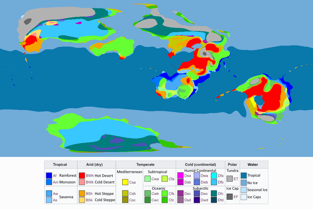
Also, as a final note: it’s generally a good idea to run some T21 models first to get a sense of the world’s climate before moving on to higher-resolution T42 or (if you’re ambitious and have a good machine) T63, but note that there can be a significant difference between models at these resolutions, especially if you’re working with more exotic worlds. My model for Teacup, for example, required 0.825 bar of CO₂ to balance at an average temperature of 16 °C at T21 resolution, but only 0.011 bar at T42 resolution. I don’t think there’s as much of a difference between T42 and T63 resolution, but I haven’t really been able to test it much.

Advanced Use of ExoPlaSim

We’ve now covered all the essential use of ExoPlaSim, and you should know enough to model most reasonable climate scenarios. But just as a point of interest, I’ll list off some options for using ExoPlaSim in ways beyond these normal cases. For now these are mostly just suggestions that you’d have to investigate on your own, but as I investigate different options in the future, I’ll update this section.

Further Posprocessor Configuration

There are a few more options for configuring the output files with the cfgpostprocessor command. In particular, it may be useful to output zonal averages (average values within each row of the climate grid, allowing you to construct a profile of some variable across latitudes). You can also limit the variables written to the output, rather than just outputting them all by default (variable codes here) which may help reduce the file sizes. Finally, rather than inputting a number of months for the times parameter, you could input a list of output times (written as fractions of the year, within paranthesis, separated by commas, e.g. (0, 0.3, 0.5, 0.7)). This doesn’t exactly match the spirit of the “months” used for Koppen zones, but it can be useful if you want to look at data for a particular part of the year (e.g., near periapsis for a highly eccentric orbit).

Constructing Atmospheric Profiles

Atmospheric layers in the output are all accompanied by a sigma level, indicating their pressure relative to surface pressure (not sea level pressure), so you can determine their value by multiplying sigma by the surface pressure in that cell. Converting atmospheric pressure to altitude is not always straightforward. The simplest approach would be to determine a scale height for the planet and construct a single altitude/air pressure function across the whole surface.

A more accurate approach may be to use the hypsometric equation to determine the vertical thickness of each layer, and add them together (with surface elevation) to determine the altitude of higher layers. The tricky bit there is determining virtual temperature; I believe using air temperature with the “liquid water content” value in the output should allow for a good approximation.

Carbon-Silicate Cycling

Generally speaking you can assume there is some level of volcanic activity that will cause the carbon-silicate cycle to balance to give you any desired level of CO₂, and then just say that your world happens to currently have that level of volcanism (though bearing in mind some general considerations for how the carbon-silicate cycle shifts as the planet evolves).

But if you really wanted to, ExoPlaSim does include options for modelling the carbon-silicate cycle. If you add “co2weathering = True” in the configure step, the program will attempt to model the rate at which CO₂ is removed from the atmosphere by weathering (there are a couple other options you can find in the documentation). Realistically you couldn’t run a model for long enough for the carbonate-silicate cycle to play out and equilibriate, but what you could potentially do is run a model until the climate balances, determine the rate of change in CO₂ based on the weathering rate and an assumed CO₂ outgassing rate, extrapolate that out for a few thousand years, and then restart the model with adjusted CO₂ levels, and iterate in that way until you reach an equilibrium in CO₂ levels. Some research along these lines has been done with earlier versions of PlaSim.

Storm Climatology

ExoPlaSim also includes options for studying the potential for hurricane-like storms to form by adding the parameter stormclim = True. This will roughly double the runtime of the model (so I recommend only turning it on after reaching equilibrium and then running for a short time), but adds some parameters describing the likelihood of storms to the output. I’m not too familiar with exactly how to interpret these, but “Genesis Potential Index” appears to be an attempt to summarize the overall likelihood for large storms to form at different points across the surface.

There are additional options to allow high Genesis Potential to trigger a “High Cadence” mode, which will record more data—in essence allowing you to track the development of individual storms—but I’m not too familiar with the process of implementing and interpreting this, and it’s unlikely to work particularly well at T21/T42 resolutions anyway.

Detailed Stellar Spectrum

Exoplasim can read from a more detailed stellar spectrum than the rough adjustment by star temperature it generally uses. To do so, use the Phoenix stellar spectrum simulation and use the commands here to convert it for use in ExoPlaSim here (to run python in command line as suggested, type in python3.6 in Konsole). You can then import it into a model using the starspec parameter in your configure command, rather than startemp.

But honestly, given the simplicity of ExoPlaSim’s internal handling of light spectra, I haven’t attempted this myself so far.

Other Climate Models

I’m not aware of any other climate models that are anywhere near as easy to install and use as ExoPlaSim (yes, all the above is “easy” by the standards of these models), and many couldn’t run in a reasonable time on a personal computer even if got them installed, but just for reference, here’s a list of others I’ve come across that may be of interest for some specific uses:

VPlanet

Not a full GCM, but a group of tools for modelling the atmospheric and orbital evolution of worlds in a variety of scenarios, with basic climate modelling—in essence, it models a world’s surface in 1 dimension from pole to pole, not a 2-dimensional grid, so it’s not as detailed or accurate but will run a lot faster (though it should actually give a more accurate estimate for the greenhouse effect of high CO₂ levels). The documentation is extensive but a bit unfocused, but there are many examples to follow and use as templates. If you don’t want to take the time to run an ExoPlaSim model, or you want to explore some scenarios outside its ability to model, this may be a good option.

ROCKE-3D

Short for "Resolving Orbital and Climate Keys of Earth and Extraterrestrial Environments with Dynamics". This is essentially the gold standard of modern exoplanet climate modelling, a comprehensive model specifically designed to avoid any assumptions specific to Earth, and adapt to a broad variety of scenarios. Unfortunately, it runs orders of magnitude slower than ExoPlaSim, and the inclusion of deep ocean circulation means it may need to simulate thousands of years rather than just decades. If you really want the best climate model available and you have access to a powerful, dedicated server, then this may be your best option.

Isca

A GCM that, similarly to ExoPlaSim, aims to be intermediate in complexity between simple models like VPlanet and advanced ones like ROCKE-3D. For the moment, it appears that the documentation and model are still under development, but it may be worth keeping an eye on in the future.

Oasis

An in-development GPU-accelerated GCM, that apparently is intended to be fairly scalable for different computers. We’ll see how the final result turns out, but it’s worth keeping an eye on.

Script Templates

To end off this tutorial, here's a couple templates you can use to create your own scripts. First, a basic script with all the configuration options available, set to Earthlike settings, so you can delete those you don't want and adjust those you do:

Here's essentially the same script but I've spaced it out a bit more and added some basic info, if you have trouble remembering what each parameter does:

And here's a script I've been working on that adjusts the script's parameters as its running to try and achieve a stable temperature within half a degree of a desired goal:

If you're using a very different planet from Earth, be sure to alter the level and adjust parameters as appropriate, and the length of the model runs. This script could also be pretty easily altered to adjust, say, flux instead of CO2 levels (by changing the modify step). The script will also save the ouput between each run, with a text file called "modelreport.txt" that allows you to keep track of how it's progressing. Note that this can end up taking significantly longer than just running to balance on the initial parameters.

That's all for now. I may continue to add more notes as I continue experimenting with different ways to use ExoPlaSim.

Buy me a cup of tea (on Patreon)