An Apple Pie from Scratch, Part VIb: Climate: Biomes and Climate Zones
 |
| Himalayas mountains, which cause a strong rainshadow effect. NASA |
Now that we’ve outlined the essential properties of our world’s global climate, it’s time to get into the particulars. For Earthlike worlds, the atmospheric convection cells should broadly determine the positions of major bands of climate—tropical, desert, temperate, tundra—but if we really want to get a sense of the weather, seasons, wildlife, and geology of a particular spot on the world—in essence, what it would be like to be there—then we have to start getting into how climate plays out locally.
This post will take some of the theory of climate we went
over last time (if you haven’t already, I strongly recommend reading at least
the first couple sections of the last post,
because they’re vital to understanding this one) and apply it as a practical
guide to mapping out the climate zones of a fictional world, with topography
and orbital features as a starting point. For this post, however, we’ll be
assuming fairly Earthlike worlds and using some tools only applicable to such
cases—that means worlds with insolation, year length, day length, obliquity,
eccentricity, size, volcanic activity, land area, pressure, and vegetation
broadly similar to Earth’s properties (about as similar as Teacup Ae is,
anyway). I will take time to address some of the more exotic cases in another
post, but let’s not get ahead of ourselves.
- Climate Zone Classification
- Step 1: Basic Sketch
- Step 2: Simulating Temperature
- Step 3: Ocean Currents and Mountains
- Step 4: Climate Bands
- Step 5: Winds
- Step 6: Precipitation
- Step 7: Climate Zones
- Impacts of Climate
- A: Tropical Climates
- B: Arid Climates
- C: Temperate Climates
- D: Continental Climates
- E: Polar and Alpine Climate
- Biomes and Biogeographic Regions
- In Summary
- Notes
Climate Zone Classification
There are, of course, many variations in local climate on
Earth, and possibly even more on other worlds, but generally speaking we can
split Earth’s surface into a handful of zones with fairly similar climate, and
so fairly similar weather and wildlife.
Now, many people tend to use “biome” and “climate zone” interchangeably
but that isn’t quite accurate. Biomes are regions with similar
ecosystems inhabited by similar organisms, and so are descriptive
regions; you have to mark them out based on the actual life present. Climate
zones are proscriptive; they’re determined by strict factors
resulting from global patterns, and so can be marked out based on a set of
rules (though we’ll have to use a bit of personal intuition here because of the
limited information and tools at hand). We can also distinguish between these
areas and biogeographic regions, which are contiguous areas with similar
enough climates and few enough barriers that wildlife can travel freely, such
that similar ecological niches tend to be occupied by related species.
Climate zones play a major role in determining biomes and
biogeographic regions, but they’re not the only factor; in the scheme we’ll
use, coastal New England and central Russia are within the same climate zone
even though they have rather different life inhabiting them. This tutorial
focuses on marking climate zones, but we’ll discuss biomes and biogeographic
regions a bit here and in following posts.
There are a variety of climate zone schemes used, but within
the worldbuilding community by far the most popular is the Köppen climate
classification system (A.K.A. the Köppen-Geiger system, as it’s a
modification of the original). This system is strictly determined by
temperature and precipitation during the warmest and coldest months (sometimes
few months) of the year, both of which can be at least guessed at based on
global climate patterns.

The Köppen system includes 31 climate zones broken down into
5 groups, but many of these climate zones are quite similar to each other or
appear only in very small regions. So to make things a bit easier, we’ll use a
reduced set of 14 climate zones.

At a glance, the impact of the atmospheric convection cells
is clear in the grouping of climate zones into horizontal belts: Lush
rainforests at the equator, giving way to savanna, steppe, and then hot deserts
at the horse latitudes, then temperate climate zones, then subarctic, and
finally the frigid tundra and ice caps.
It’s also pretty clear that topography has a big impact:
high plateaus like the Himalayas and Rockies create cold deserts and even
tundra zones far from the poles.
But there’s definitely more at play here: these climate
belts appear slanted across the continents, and some appear only on certain
sides; mediterranean and oceanic climate zones are mostly restricted to the
west coasts of continents, and subtropical zones to the east coasts.
That’s the subtle variation we want to reproduce here; not
only in pursuit of realism, but also to give our worlds a bit of diversity and
help guide the development of lifeforms and societies later on.
Before we start, I’m assuming you already have at least a
basic sketch of your world’s landmasses and topography. We don’t need anything
too detailed just yet. If you haven’t gotten that far, I’ll refer you back to
my guide to constructing a tectonic history. I suggest using an equirectangular
projection for the map, as it accurately represents cardinal directions
without distorting shapes too much; gplates can export such maps (it calls them
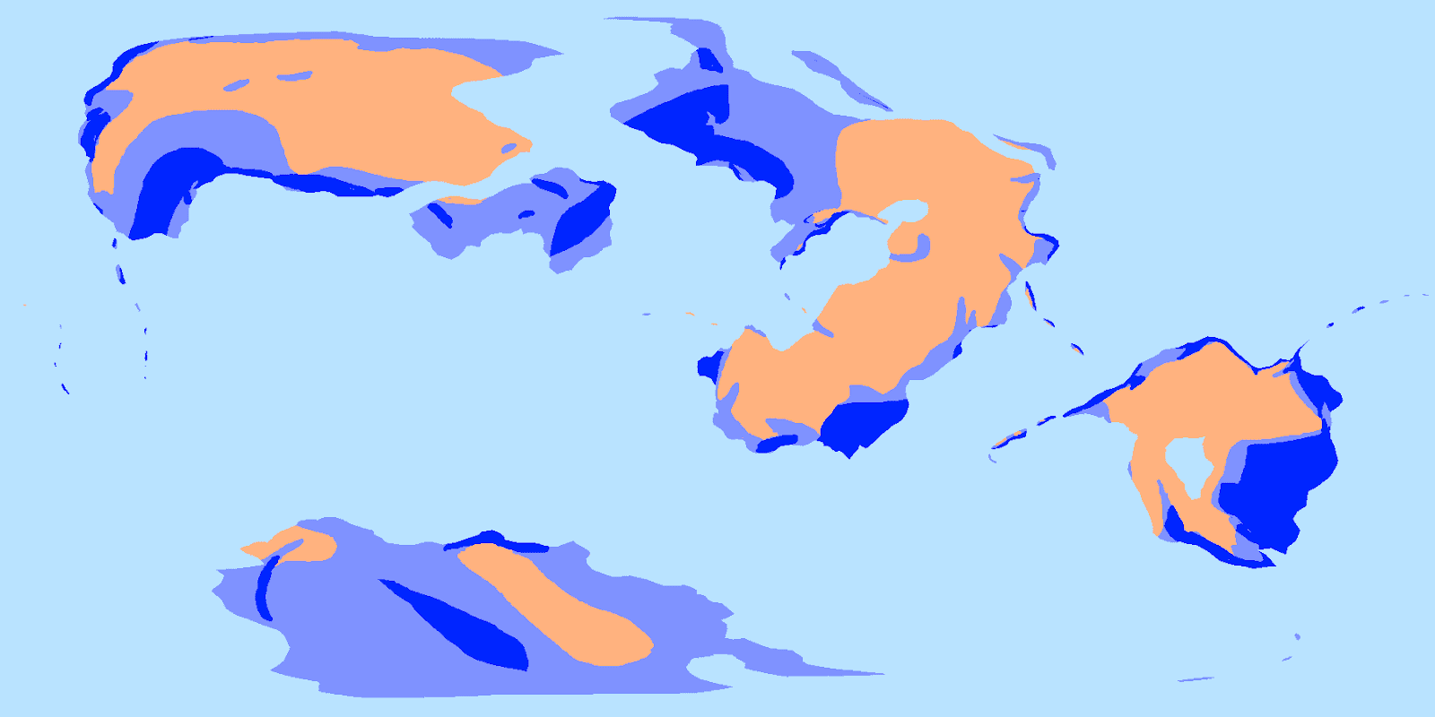
just “rectangular”). Here’s what I’m working with in the case of our example
world, Teacup Ae (with the interim names of the continents and oceans, for
reference):

However, east-west distances near the poles are pretty
distorted on this projection, so I suggest you have Gplates open as well in the
globe view, and use the measurement tool there when judging distances from the
coasts (Even if you didn’t build your world map in Gplates, you can import any
equirectangular map as a raster). Maptoglobe is also a
decent option.
I’m also assuming you’ve picked out the orbital parameters
that will determine your world’s seasonal cycle; obliquity, eccentricity,
and argument of obliquity. If you’re unfamiliar with the terms, I
defined them in Part III;
I’ve also discussed their impact on habitability
and global climate,
and built the “Irradiance Fast Rot” tab in my spreadsheet
to give you an idea of what impact particular parameters will have. I initially
defined these values for Teacup Ae as 15°
obliquity, 0.1 eccentricity, and 150° argument of obliquity, but in the course
of making this tutorial I’ve found the need to tweak them a bit to get results
I liked—so don’t be afraid to do the same yourself.
And finally, I will assume that these planets all spin
towards the east, as Earth does. If your planet spins west and you want
to avoid getting confused over the course of this tutorial, you can flip your
map horizontally or rotate it 180°,
proceed through the tutorial, and then flip or rotate the map back at the end
(if you don’t like the climate map at the end of this tutorial, flipping the
map is also a useful way to get a different climate without needing new
landmasses and topography).
Step 1: Basic Sketch
To start off with, we’re going to need at least a basic
sketch of some major types of land cover: Desert, ice cap, dense forest and
more open grassland and shrubland. These are, of course, determined by the
climate, so it may seem like a catch-22 to have to use them to work out the
climate, but this is only a sketch; it doesn’t have to be perfect, and if you
like you can iterate this process by taking the final climate map and using it
to start the process over, tedious though that may be.
Prevailing Winds
To make our sketch, we’ll use the boundaries of the
atmospheric convection cells and the prevailing winds they produce. Though, as
we’ll see, these winds move with the seasons, in this case we’ll use a
simplified model where they’re tied to latitude, and we’ll also assume that
Teacup Ae’s rotation rate is similar enough to Earth’s for the cell boundaries
to be at roughly the same latitudes.
In that case, we can mark out alternating easterly and
westerly prevailing winds like so:

As expected, we have converging winds at 0° and 60° latitude, which should create wet forest belts, and diverging winds at
30° and the poles, which should make dry desert belts and polar tundra. We also
have alternating easterly and westerly prevailing winds; onshore winds
blowing from sea to land will carry moisture far inland, while offshore
winds will leave the land relatively dry.
Ice Caps
Let’s mark out these
regions first, where ice persists year-round: Exactly how far they extend on
flat land depends on the particular global climate state—which is to say, you
can put the boundary about anywhere you want, but once it gets past around 40°
latitude you might be approaching the point where we’d expect a rapid
transition to a snowball state.
The ice caps will
extend further equatorward in mountains. The general rule of thumb is that 1
kilometer increased altitude is similar to moving 8° poleward, but distance
from the coasts matters as well; glaciers will advance further equatorward on
inland regions that are better insulated from the moderating influence of the
oceans. On the other hand, landmasses at the poles totally isolated from other
continents by oceans will be more likely to freeze over completely. These sorts
of differences in topography can lead to major asymmetries in the extent of ice
caps in either hemisphere.
So here’s how that
looks for Ae, with ice caps similar in size to Earth, though without isolated
landmasses like Antarctica or Greenland. Note that I’m only marking ice caps on
land here; they will extend onto the seas as well, but for this process we
don’t need to worry about that.

Deserts
Next up, desert regions which have little or no rain and
vegetation. The main belt of deserts will be near the horse latitudes, though
centered a little closer to the equator; on Earth they’re mostly between 15° and 30° latitude, but they’ll move with
widening or shrinking of the Hadley cell on other worlds.
They don’t occupy
all land at these latitudes, though; onshore winds keep east coasts at these
latitudes wet, reaching inwards around 1,000-1,500 km or to a substantial
mountain range. Monsoon winds can also bring moisture into the desert belt;
we’ll discuss the mechanisms behind them later, but for now suffice it to say
that large landmasses in the horse latitudes directly north or south of
equatorial oceans will tend to have wet coasts and smaller deserts.
Outside of the Hadley cell, winds are less regular so there
are no coastal deserts even where offshore winds occur. But deserts can still
occur here—or near the equator—out of reach of moist winds from the oceans.
One way is simple distance; air moving over land will be
continuously precipitating out water and so have less and less remaining as it
moves further inland, so forest and grassland gives way to steppe gives way to
desert. This should occur around 2-3,000 km away from coasts with onshore winds
and 1,000 km away from coasts with offshore winds (these distances may be
different on planets with different average levels of wind speed or
precipitation). Bear in mind that when I say “coasts” I’m referring to those on
major oceans, not every minor inlet or small inland sea.
The other way is with orographic lift: When
water-laden air encounters a mountain range, it is forced upwards and the
surrounding pressure drops; the air thus expands and cools, and the water vapor
contained in it condenses and rains out. This means high rains on the windward
side of the mountains, but little moisture left for the leeward side, or
anywhere else downwind. The descending air also condenses and warms, creating a
hot, dry wind that further contributes to the leeward side’s aridity. Large
mountain ranges can thus create a rainshadow, with a sharp division
between lush upwind forests and bare downwind desert.
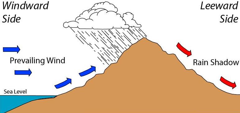 |
| Meg Stewart, Wikimedia |
Even fairly low mountains can cause orographic lift when
facing consistent winds,
but generally speaking it becomes significant at the scale of continents when
average relief, height of a mountain range about the surrounding
terrain, exceeds 1 km, and can create rainshadow deserts when relief exceeds 2
km. But in particular cases the impact can depend on the moisture content and
strength of the winds, which will depend on distance from the sea and the wider
context of atmospheric precipitation; a range on the equator facing onshore
winds may need to be over 3 km high to cause a rainshadow desert, while one far
inland at higher latitude may only need to be 1 km high.
On the windward side of the mountains, rains generally peak at
1-1.5 km relief, which can make these areas wetter than you might expect
without the mountains, in some cases even wetter than areas closer to the sea.
“Stepped” slopes with flat areas between sections of high relief can allow
moisture to reach higher altitudes, but in general you can expect anywhere
above 4 km to be dry.
All that in mind, here are Teacup Ae’s deserts:

Dense Forest
Much of the temperate areas of the planet will have some
amount of forest cover (assuming an Earthlike biosphere), but we’re more
concerned with rainforests and similarly lush coastal forests (this is because
what we’re ultimately concerned with in the next steps is albedo).
First off, there should be a belt of rainforest circling the
world within 10° latitude of the
equator. It won’t appear everywhere; regions at high altitude, thousands of
miles from the coasts, or affected by rainshadows will lack them. But anywhere
near the coasts, even with offshore winds, should sport thick forests. They
will tend to extend further poleward and inland on eastern coasts with onshore
winds, though.
Outside of this
rainforest belt, dense forests don’t encircle the world at any points, but do
still occur in areas with high rain. This will be mostly islands or coastlines
with onshore winds, especially those directly exposed to large oceans. You can particularly
expect large forested regions at about 45° to 60° latitude on western coasts.
We also have to
take orographic lift into account: Rainshadows will inhibit forest growth, but
high rains on the windward sides of mountains will encourage forests. A large
mountain range can create forests well inland of where you might normally
expect them (especially if it’s a young mountain range laden with nutrients).
And so here are
these various forest types on Ae:

Any remaining land we’ll
assume is scattered or less lush forest, shrubland, and grassland.
This process of
sketching out the climate can be pretty quick once you get used to it, so you
may find it useful on its own any time you’re not concerned with the
particulars of local climate. For example, this is how I produced those
paleoclimate maps in the last section. But for those of us looking for detail,
we can use this as a starting point for the next step.
Step 2: Simulating Temperature
For this step we’re going to use a convenient but remarkably
little-known piece of software called Clima-Sim
(the free “demo” version is sufficient for our uses). This program can do most
of the work for us of determining surface temperature across the seasons,
accounting for atmospheric circulation, insolation, surface albedo, and
topography. It even has basic modelling of clouds, ocean currents, and snow/ice
accumulation. It’s not the most advanced model out there—the GCMs that climate
scientists use (“Global Climate Model” or “General Circulation Model” depending
on who you ask) are pretty inaccessible for anyone not familiar with FORTRAN—so
it can’t predict precipitation and doesn’t do too well with exotic cases, but
it’s a big step up from just guessing temperature ourselves.
Planet Parameters
Once it’s downloaded and started, it’ll need a bit of setup.
We’ll start with the settings menu.
“Settings” -> “Terrestrial” will open up a menu
regarding various greenhouse gasses and similar forcings. The free version
doesn’t let us play around with all these settings too much, but we can choose
from several presets. The default, “1951-1980 AD”, represents Earth’s
climate just before the major rise in CO2 levels and has a global
average temperature of about 15 °C
with Earth’s topography.

The help menus can tell you about the other settings, but
the two most notable are “Cretaceous (90 million yr ago)” which is about
9.5 °C warmer, and “Last
Glacial Max (18000 BC)” which is about 5 °C cooler. These are convenient presets for hothouse and icehouse
glacial climate states.
“Settings” -> “Orbital/Astronomical” allows us to
alter the main forcings determining our seasons—in particular, “Axial tilt
(degrees)”, “Orbital eccentricity”, and “Date of perihelion”.
Clima-Sim uses an idealized 360-day year with 30-day months and the winter
solstice at January 1, so find the mean anomaly of the periapsis from the
winter solstice (it’s 180°
offset from the argument of obliquity, which I use in my spreadsheet), divide
that by 30 to determine the month (1 = January, 2 = February, etc.), and multiply
the remainder by 30 to determine the day. Though we can set these values
however we like, Clima-Sim’s limited circulation model makes it unsuited for
high obliquities or eccentricities.

“Semimajor axis (A.U.)” only affects insolation, not
year length; it can be used to adjust average global temperature, but doesn’t
reflect the stronger seasons of longer years. “Hours in solar day” only
affects the daily range of temperatures, and not atmospheric circulation or year
length.
Terrain

Clima-Sim uses a fairly low-resolution grid of cells (1296
at most) for its simulation, to help limit computation time. Each cell
represents the same area of the surface (hence the “stretching” towards the
poles) and we have to specify a dominant surface type and elevation for each
cell, though there is some interpolation between cells in the simulation.
When you erase the continents, all cells default to water
(which includes ice sheets over water), so we have to draw in land areas in the
4 land surface types that we sketched out in the last section: Permanent Ice,
Dense Forest, Grass, and Desert. Clima-Sim uses these to
determine albedo.

There are 4 levels of elevation, which must be specified after
placing surface types: land areas will start by default as fairly flat
(0-1000 m), and we have to draw in areas of low mountains (1000-2000 m),
medium mountains (2000-4000 m), and high mountains (>4000 m). These
are used to determine air flow and surface temperature.

Conveniently, Clima-Sim allows us to import a map and
display it as a background to the map screen, to help draw new continents. To
do this:
- Open your equirectangular map in your image editor of choice (paint.net is my go-to).
- Resize the map to 720 pixels wide by 420 pixels tall.
- Save this as a .bmp or .jpg file (any name will do) and place it in the “clima-sim” folder.
- Open Clima-Sim
- Select “Erase Continents”
- Select “Display” -> “Use imported background map (toggle, off and back on for new selection”
- Select your map file

You can then use this map to fill in Clima-sim’s grid
However, the free version of Clima-Sim doesn’t allow you to save new
topography, and is also somewhat prone to crashing (in particular, avoid
dragging the cursor from inside to outside the map area with the mouse button
held down while drawing terrain). So to save some frustration and ensure
consistency across sessions, I suggest determining these terrain types outside
Clima-Sim. For your convenience, here’s a rough copy of the grid the program
uses:

Overlay this on your resized map, and fill it in with
high-contrast colors to create 2 maps: One for surface type and one for
elevation. In each case you’re trying to represent the dominant terrain in most
of the cell, though it may be worth exaggerating isolated islands or mountains,
or substantial features that cross multiple cells but don’t occupy the majority
of any one. For reference, you can open up Clima-Sim and select “Display”
-> “Draw world map outline (toggle)” to see how the default terrain grid
compares to Earth’s topography. Note how New Zealand is large enough to merit a
cell of land, but Hawaii is not.

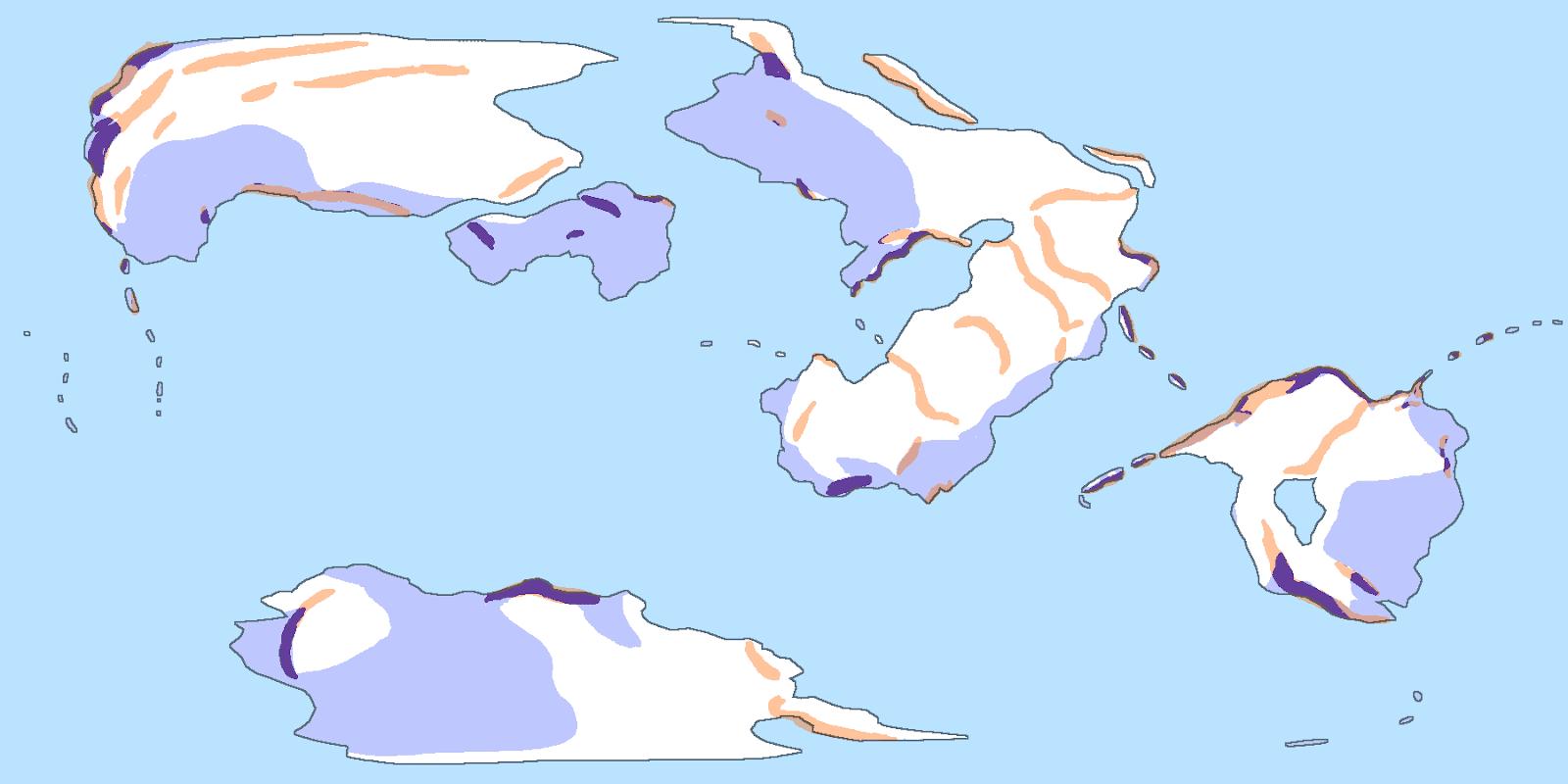
For Ae, here are my grids for surface type (top) and
elevation (bottom) (after adjusting the ice caps to match the simulation, as I'll describe in a moment):


So now the process of drawing terrain is:
- Erase Continents
- Import surface type map
- Draw surface types (water is the default, so we only need to draw land types)
- Import elevation map
- Draw elevation (again, fairly flat is the default, so we only need to draw mountains—if you misclick and place mountain on a cell that should be flat, placing down a surface type again should reset the elevation).
Simulating Climate
Input your terrain, make sure you’ve input the right orbital
parameters and selected the right preset for forcings, toggle off the imported
map so it’s not in the way, and now we are finally ready to begin the climate
simulation. To do so, make sure that “Run mode” is set to “Full run
(does three above in order, initialized with zonal temperatures)” and press
“Start Model Run” in the upper right corner.

Once the run completes, it will display average annual
temperatures at sea level. We should make a couple adjustments first to ensure
accuracy:
- Select “Options” -> “Elevation options” -> “Show actual surface temperatures”. This will display temperatures adjusted for elevation, with temperature dropping by 4.46 °C per kilometer of elevation above sea level.
- Select “Options” -> “Isotherm Quality” -> “High (slow but smooth)”. Fairly self-explanatory.
Near the center of the controls is a dropdown menu for
different months. This may be worth playing around with a little, but the most
important months are July and January (2) (the January at the end
of the simulation, not the start), which have their own shortcuts below this
menu. These should represent the seasonal extremes—summer in the north
and winter in the south for July, and winter in the
north and summer in the south for January (2)
(worlds with high eccentricity and periapsis not aligned with a solstice may
have different seasonal peaks; right-click on the map somewhere in the mid
latitudes to see the local temperature curve across the year, and survey
multiple such locations to get a sense of the seasonal peaks across the
planet).

The first time you run the model, you should check how the
distribution of ice caps compares to the summer temperatures in each
hemisphere. There should be no land cells below 0 °C without permanent ice, and no cells above 0 °C with permanent ice. If
there is a mismatch, alter the initial surface type map and rerun the
simulation (as the initial albedo of ice will affect the final outcome), and
iterate until ice distribution matches modelled surface temperature.
Similarly, there
shouldn’t be any dense forests in cells below 10 °C in summer—though, as we’ll
see, Clima-Sim isn’t totally accurate for some coastal temperatures at high
latitudes, so there’s a bit of leeway here for western coasts.
If you find that
you don’t like the distribution of ice (and you may also want to peak ahead a
couple sections to the climate bands to get a sense of how they’ll turn out)
then you can adjust obliquity and eccentricity to alter the seasonal cycle, or
adjust insolation (by adjusting the model’s semimajor axis) to alter average
temperature for the whole planet.
In the specific
case of Teacup Ae, I found the original parameters resulted in large areas of
Steno and Hutton that remained cold year-round and would have ended up as
tundra, so I’ve decided to increase obliquity to 25°, and move the argument of
obliquity to 120°—expanding the temperate and continental climate bands,
especially in the northern hemisphere (I also increased the semimajor axis to 1.01,
which reduced the average global temperature to about 16 °C).
Exporting Maps
Once we’re happy with the overall global temperature
distribution, we should export the temperature maps for the next steps. Every
time you generate a new map with Clima-Sim (usually by changing the month
displayed) the map displayed is automatically saved as “lastmap.bmp” either in the “clima-sim”
folder or in the same directory as the map overlays you imported. When you’ve generated a temperature map you
want to save, you can rename this file (open it first to confirm it’s the map
you want), and the program will generate a new file for the next map without
altering the renamed file.
The default maps are a bit cluttered, so I like to select “Display”
-> “Isotherms only” and “Options” -> “Isotherm color” ->
“Black”, then import a blank white image as the background. This lets me
display an image of just the isotherms (lines of equal temperature), that I can
then overlay on more accurate maps of the landmasses of Ae:
| Note that the program adds an extra line of pixels to the bottom. |
These isotherms don’t extend all the way to the edges of the
map, and will probably have some odd gaps, so keep Clima-Sim open as a
reference for marking out temperature zones.
You can also use “Options” -> “Isotherm spacing”
to alter the temperature step and numbers of isotherms.
We’ll need at least 4 maps for the process of marking out
climate zones:
- 2 maps with medium isotherm spacing for both of the seasonal peaks (typically July and January (2)).
- Having maps with wide isotherm spacing for the seasonal peaks is convenient as well.
- For each hemisphere we’ll also need a map with wide spacing either 2 months before or after peak summer (whichever is warmest at high latitudes where the mean annual temperature is around 10 °C).
- Having a mean annual temperature map may be cool as well, though not necessary for this tutorial.
I’ll trust that you can figure out the process of resizing
these maps back to equirectangular (2:1 width/height ratio), smoothing out the
isotherms, converting them to temperature zones, and filling in the edges of the
map—it’s mostly just an elaborate process of filling in the lines or
interpolating between lines. If you want to stay fully realistic, there should
be only one temperature zone across the entire top and bottom boundaries, as
these represent points, and temperature zones should wrap around the left and
right edges.


Step 3: Ocean Currents and Mountains
A special note: I’m doing this step before marking climate bands because I want to have consistent temperature maps, but if you don’t care about that then it may be easier to do this after Step 4, because there are less boundaries to worry about.
Clima-Sim does a pretty good job of simulating global
climate, and it does try to account for ocean currents, but ultimately it comes
up a bit short. Below is a comparison between the average temperatures modeled
by Clima-Sim for Earth’s topography, and the actual recorded temperatures for
1951-1980 (the period used to calibrate Clima-Sim), showing discrepancies at
high-latitude coastal areas of 10 °C
or more (in the northern hemisphere, at least; the south has little land area
at the relevant latitudes):
 |
| Blue areas are warmer in reality than simulated, red areas are cooler. |
Compare that with
Earth’s dominant ocean currents, which carry warm waters poleward in some areas
and cool waters equatorward in others:
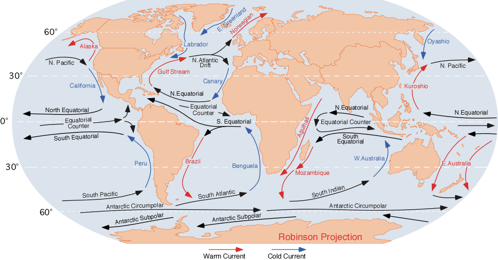 |
| Dr. Michael Pidwirny |
Drawing Currents
Now, just to
prevent some confusion: if you’ve spent some time on worldbuilding forums or
watched this video, you’ve probably seen current maps that
look something like this:

Simply put, this map isn’t actually depicting currents. They
don’t stick quite that close to the coasts, and they don’t take hard turns to
shoot straight across the oceans. This is more of a depiction of the effects
that currents have on land. It’s typically used as a heuristic for determining
climate zones without the need for temperature or precipitation data, and in
that sense it works well enough, but many people—unaware of the abstracted
nature of these maps—often get caught up trying to work out the mechanics of
minor coastal features, when in reality they’re not that important to global
climate. As I’m using ocean currents more narrowly to adjust temperatures in
certain regions, I can stick with a more direct depiction of their actual
paths.
In every ocean a single current, the equatorial
countercurrent, flows east, generally sticking close to the equator but
deflected somewhat by coastlines at a low angle to the current’s direction of
flow.

Once this current hits a coastline (or a large archipelago)
that’s more perpendicular, it splits and curves around to two currents, the equatorial
currents, flowing west, around 5-10°
latitude north and south of the countercurrent.

These flow back across the ocean. Some water begins curving poleward
within a couple thousand kilometers of leaving the coast, but the main currents
will be where the countercurrents encounter the eastern coasts of a landmass
along the equator, or where a landmass lies directly to the north or south
within about 50° latitude.
 |
| Typical current patterns. |
These currents then flow poleward along the coasts. They
don’t flow too close to the coasts, mind; the main flow is often several
hundred kilometers offshore, and the currents won’t sweep into bays and coastal
seas. There are currents circulating in these areas, but over such short
distances they perform too little heat transport to be relevant to climate. We
can think of these bodies of water as “inheriting” the heating or cooling
effect of whatever current flows past any seaways connecting it them to the
oceans. This is true even where there is an open east-west seaway between continents;
some water will flow through, but the main poleward current will continue.
Similarly, a parallel north-south seaway between a large landmass and an
offshore island can have a side current flowing through it and rejoining the
main current.

This is not to imply that straits have no impact at all; in some cases they can provide a passage for warm currents into areas that would otherwise be affected only by cold equatorward currents.

These currents bring warm equatorial waters poleward, so we’ll mark them as warm currents.

These currents bring warm equatorial waters poleward, so we’ll mark them as warm currents.

The poleward currents continue along the coasts through the
Hadley cells, but on entering the Ferrel cells the combination of the Coriolis
effect and westerly winds start pushing them east. They separate from the
coasts at around 40-50° latitude,
depending on the angle of the coastlines (more straight north-south oriented
coastlines will cause more poleward separation) and then turn east across the
ocean. They’ll generally keep a slight tilt poleward, though they can curve
equatorward to meet the poleward tip of a continent that extends partially into
the Ferrel cell from the Hadley cell. These currents still carry water warmer
than surrounding waters, so we’ll keep them marked as warm currents.

Once this current encounters
a coast, it will split again: one branch will flow along the coasts equatorward
and merge back with the equatorial current. The other flows poleward along the
coast. Similarly to before, we can also expect an equatorward current wherever
the eastward current passes poleward of an equatorial landmass.

The poleward
current is still warm relative to surrounding waters, but the equatorward
current is now carrying relatively cool water towards the equator, so we’ll
mark them as cold.

If no landmasses
block the poleward current (or sea ice, which forms where the sea remains below
-2 °C in summer and does just about as good a job blocking surface currents),
it will continue to around 80° latitude, where the polar easterlies will cause
it to curve back west until hitting a coast (again, possibly curving slightly
equatorward to meet one if necessary), and then flow equatorward to merge with
the mid-latitude currents. If the pole is open water, you can expect a small
circumpolar current flowing west around the pole, though this has little impact
on temperature.
There are a few key
patterns that emerge here. For one, there is circulation throughout the ocean;
nowhere does a current flow into a body of water without there being
another current flowing out.
Another is the
formation of large circulation cells, like in the atmosphere—but in the oceans
they’re known as gyres. Gyres should form off the west coasts of all
large landmasses at low latitudes, turning clockwise in the northern
hemisphere and counterclockwise in the south.
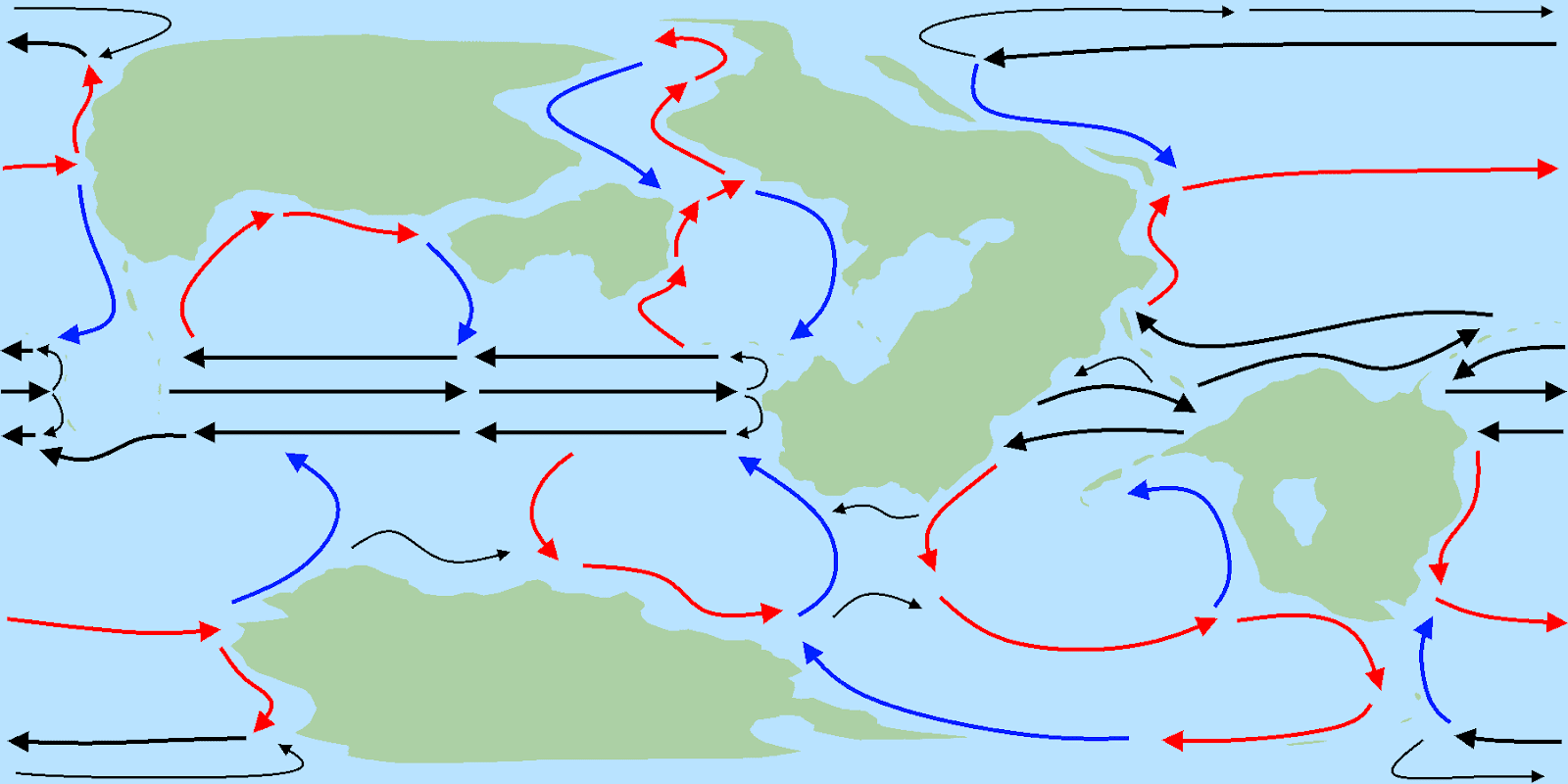
Of course, even this is an abstraction of currents to some extent. Water is in motion all across the ocean, and a complete map of surface currents would look something more like this:
But this method does represent the main flow of currents, while hopefully being intuitive enough to chart out for your own worlds.
Of course, even this is an abstraction of currents to some extent. Water is in motion all across the ocean, and a complete map of surface currents would look something more like this:
 |
| NASA/Goddard Space Flight Center Scientific Visualization Studio |
But this method does represent the main flow of currents, while hopefully being intuitive enough to chart out for your own worlds.
Currents and Temperature
To have an impact on climate, currents need to move pretty
far poleward or equatorward, something like 30° latitude or more—but they’ll retain their heating or cooling effect
when crossing the ocean. This means the temperature effects should only be
significant where there are large, uninterrupted oceans or major channels extending
far across latitudes. This also means that the warming or cooling effect of a
current is not lost the moment it changes directions; a poleward current that
turns equatorward will still warm the nearby coasts, until it moves more than
around 10° latitude and the water temperature begins to approach the
surrounding land temperature.
Starting with
Clima-Sim’s output, the biggest impacts will be at around 50-70° latitude:
western coasts here will be warmer thanks to poleward currents, and eastern
coasts cooler due to equatorward currents. Per Earth’s example, the former
effect seems to be slightly stronger; the difference between Clima-Sim’s output
and the adjusted temperature should peak at around 15 °C warmer on west coasts
and 10 °C cooler on east coasts at close to 60° latitude for both. Closer to
the equator, some minor heating of eastern coasts and cooling of western coasts
at 20° latitude is reasonable, but it shouldn’t be a huge change from
Clima-Sim’s output.
 |
| Areas of temperature adjustments for currents: red areas will be made warmer and blue areas made cooler. |
At the equator
there will also be heating of eastern coasts by the equatorial currents, moreso
the farther these currents have traveled. These currents pick up heat as they
travel west, and it can build up on the western side of the ocean over several
years until it causes a temporary reversal of prevailing winds to carry heat
back east. In the Pacific these are called “El Niño” events and occur
about every 5 years, warming South America and cooling Australia. These events
are too subtle and infrequent to be worth accounting for in this tutorial
(except perhaps to inform distribution of coral reefs), but may be worth
keeping in mind as a likely feature of any broad equatorial oceans.
All that in mind,
here are the adjusted temperature maps for Ae:


Mountains
One last adjustment we can make is to mountain temperatures.
The low resolution of Clima-Sim’s simulation grid means that it may not quite
reflect the shape of high-elevation cold zones accurately, so you’ll have to
make some adjustments for that.
 |
| Typical Clima-sim output for a mountain range (left) and more realistic adjustment (right) |
It also seems to slightly overestimate temperatures on high
mountains: If you have any large plateaus above 4 km elevation, their interiors
should have average temperatures below 10 °C.
And so, at long last, here are the final temperature maps
for Ae (with contour lines at 1 km increments):


Step 4: Climate Bands
The temperature data we’ve gathered is enough to mark off some
of the groups in the Köppen scheme—what I’ll refer to as the planet’s climate
bands. The procedure is fairly straightforward: Take the temperature maps
from clima-sim (with adjustments for ocean currents and mountains, if you’re
doing that before this step), overlay them on a map of your world, and starting
from the equator mark out all land areas above the given temperatures for each
band in summer or winter, as specified.
Actually, rather than starting with the geographical equator,
let’s mark the thermal equator for each season: This is the line near
the equator with the highest temperature in each line of longitude. If you’ve
got a lot of high terrain near the equator it might get a pretty jagged, but
that’s alright for now.


Next, mark off the regions in each hemisphere which are at
least 18 °C in winter.
This is the tropical band, with
Group A climate zones.

Next, in the remaining area mark off the regions which are
at least 0 °C in winter.
This is the temperate band, with
Group C climate zones.
(On further review of Koppen climate zones, it appears that you should then remove any areas within this band that are less than 10 °C in summer, as these areas will be tundra. In most cases this should only appear in some equatorial mountain ranges).

Within the temperate band, mark off the regions which are at
least 22 °C in summer. These are the hot-summer zones of the temperate band;
remaining temperate regions are cool-summer
zones.

Next, in the remaining area mark off the regions which are
at least 10 °C in summer.
This is the continental band, with
Group D climate zones.

Within the continental band, take a time 2 months before or after peak summer
(whichever is hottest) and mark off regions which are at least 10 °C. This is the humid continental zone; remaining continental regions are the subarctic zone.

Next, in the remaining area mark off the regions which are
at least 0 °C in summer.
This is tundra, the ET
climate zone.

The remaining area, which is below 0 °C even in summer, is ice cap, the EF climate zone.

That settles the land climate bands, but while we’re here we
can also mark off a couple of informal climate areas at sea:
Areas above 18 °C
in winter can support coral
reefs in shallow waters (presuming the temperature limits are the same as
for reefs on Earth).

Areas below -2 °C
in summer will have permanent
ice sheets.

Remaining areas below -2 °C in winter will have seasonal ice sheets.

All this is enough to give us a general idea of the planet’s
climate, and it’s at this point that we should decide whether to commit to this
climate or restart with altered orbital characteristics or topography. If
you’re in a hurry, you could stop here and try to determine climate zones by
general location rather than simulating winds and precipitation; but for this
tutorial, we’ll carry on to the end.
Step 5: Winds
 |
| Typical seasonal temperature (top), air pressure and winds (middle), and precipitation (bottom). (the original page where I got these animations has disappeared but is archived here and versions interpolated to higher resolution are also available here) |
Further subdivision of Koppen climate zones requires
precipitation data, which Clima-Sim doesn’t provide. Precipitation on Earth mainly
originates in the oceans: water evaporates in warm seas, is carried inland, and
then—if conditions are right—condenses and falls onto land. Sussing out the
connections between temperature, pressure, wind, and precipitation can be
tricky, and—as I’ve learned my self—trying to find simpler shortcuts can often
have very misleading outcomes. But we’ll take it all step-by-step.
(When first published this tutorial contained a much
different version of the next few sections. In retrospect, the methodology
employed there was both too simple in concept and too complex in execution.
This new approach sacrifices some precision—I’m leaning much more heavily on
your personal intuition and artistry to divide up certain zones—but hopefully
makes up for it in accuracy in more closely modelling the actual mechanisms of
global climate).
Global Circulation
To start, we’ll mark out the likely location of the ITCZ
in summer and winter. It should roughly follow the thermal equator, but a
little more smoothed out so it’s not zigzagging through mountain ranges.
Compare Earth’s seasonal thermal equators and ITCZs for reference:
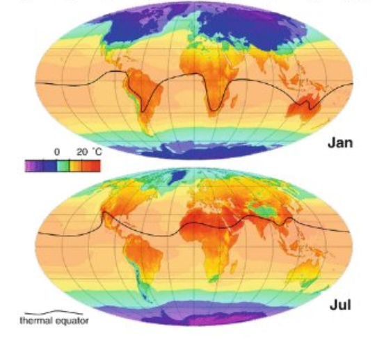
 |
| Top: Seasonal temperature and thermal equator. Richter 2014. Bottom: Seasonal ITCZ. Mats Halldin, Wikimedia. |
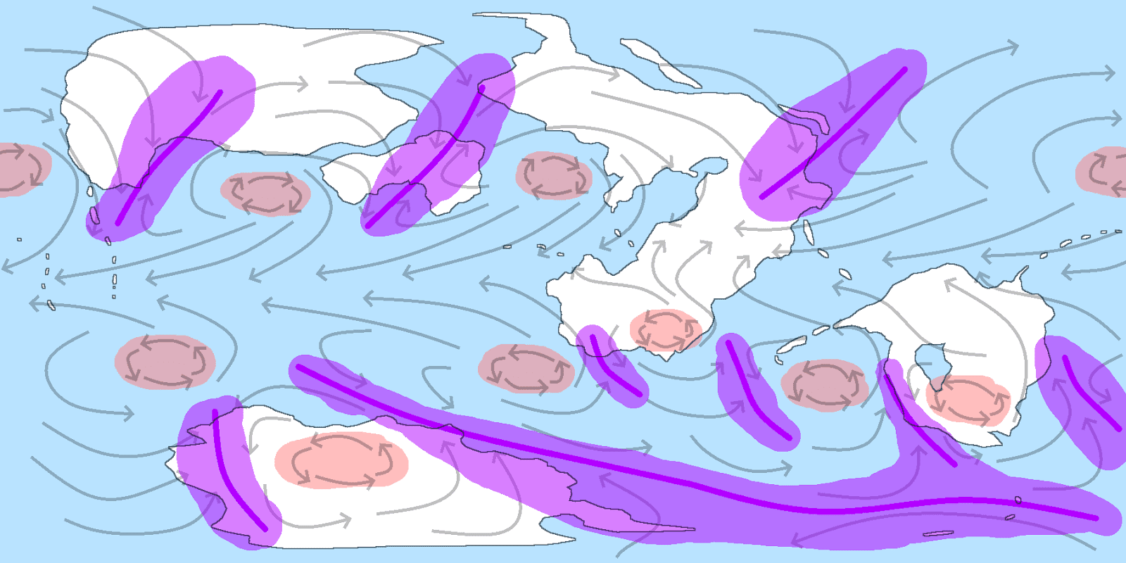
Here’s how I’ve marked them out for Teacup Ae (blue is the ITCZ, red is the thermal equator):

The tropical easterlies flow towards the ITCZ, not the equator, so as the ITCZ moves with the seasons the prevailing winds in the regions it passes over will switch direction. This is the primary cause of monsoon winds: onshore winds in summer bring rains, and offshore winds in winter cause dry conditions.
The further we get from the equator and towards the poles,
the more our neat model of convection cell boundaries and prevailing winds
becomes a suggestion rather than a law. Rather than a single high-pressure belt
at the horse latitudes, we instead find a number of distinct subtropical
highs.
These tend to be strongest over cold areas, so they’re best
identified by patterns of ocean currents. In the current map you made back in
Step 3, you should find a number of large ocean gyres between around 10° and 50° latitude, turning clockwise in the northern hemisphere and
anticlockwise in the south. The cold, equatorward legs of these currents—which
should lie along the western coasts of major landmasses—will create our
subtropical highs, just offshore to the west. Like the ITCZ they’ll shift with
the seasons, but more subtly; place them a bit further towards the equatorward
side of the gyre in winter (centered around 25° latitude, depending on the
overall extent of the gyre) and a bit towards the poleward side in summer
(centered around 35° latitude).
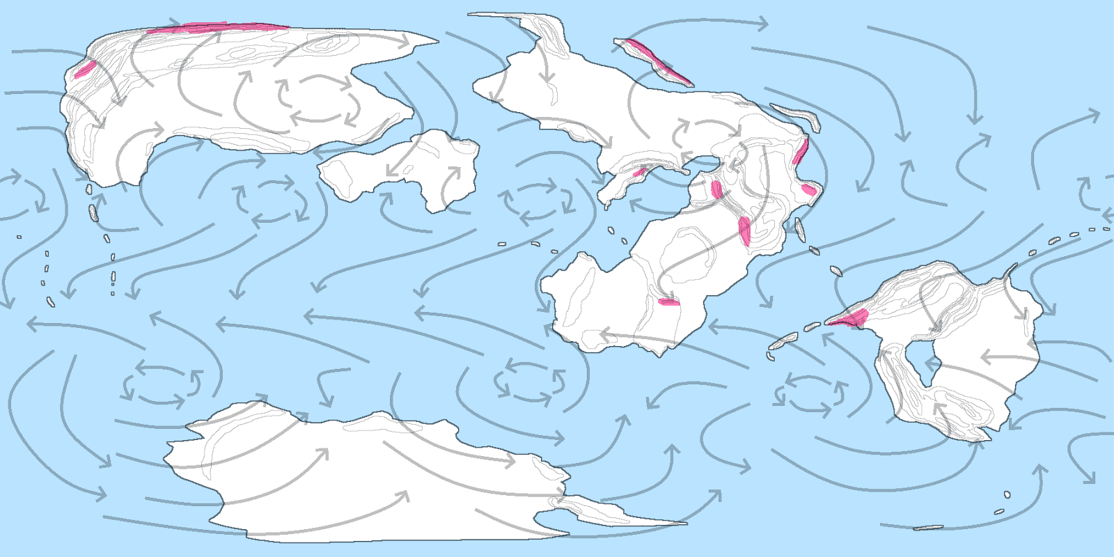
Here they are for teacup, marked in red (with currents shown as well).


- A landmass is large enough to support such a high-pressure zone if it’s significantly cooler (~5-10°) than oceans at the same latitude.
- Multiple nearby landmasses without warm oceans separating them can be counted as one landmass
- The high-pressure zone will appear roughly in the center, but shifted towards any particularly cold regions (relative to latitude) such as large mountain plateaus.
- They’ll generally be a bit further poleward than the ocean subtropical highs, and can even appear on landmasses near the poles.


If we wanted to, we
could dig further into patterns of pressure and add low-pressure zones (which
seem to form over continents in summer and high-latitude oceans in winter) but
the rules there are even more vague and these high zones are sufficient to get
a pretty good sense of prevailing winds.
Prevailing Winds
Prevailing winds are, as in the idealized models we’ve
looked at before, a product of pressure and the Coriolis effect. Winds tend to
blow from high to low pressure zones, but the Coriolis effect causes winds
blowing north or south to deflect from a straight path; to the right in
the northern hemisphere, and to the left in the southern
hemisphere. On a world covered in homogenous ocean, this would create the
neat convection cells of those models, but on a world of mixed continents and
oceans we get a more complicated jumble of winds that bears some overall
resemblance to the idealized case but deviates from it in many places.
To start off, we can mark the anticyclones. These
appear over high-pressure zones as air moving down its pressure gradient is
curved by the Coriolis effect. Though the path of a lone object in a vacuum
might only be gradually altered by this effect, the interaction of many air
masses on Earth accentuates the effect until air no longer moves directly out
of highs but instead spirals tightly around them; turning clockwise in
the northern hemisphere and counterclockwise in the south
(same as the underlying ocean gyres). We’ll just mark winds in the cores of
these anticyclones for now, and build them out from there:


Next, we’ll mark out the trade winds, or tropical
easterlies, which dominate in the tropics. For the most part, they do
actually behave as in the idealized models; blowing equatorward and curving
towards the west until they meet at the ITCZ blowing nearly directly west. But
there are a few wrinkles.
The trade winds mostly originate from the subtropical highs,
so the position of these highs influences how steeply the winds approach the
ITCZ, and where it passes before then. On the eastern sides of the highs, it’s
typical for a wind to begin moving east and then curve around to the west.
You should have some winds crossing the equator from the
winter hemisphere to the summer hemisphere. When this happens, the influence of
the Coriolis effect switches direction, so rather than curving to the west,
winds will curve to the east—and they can do so quite quickly.
Tall mountain ranges have a subtle effect on winds,
corralling but not blocking them. Think of it like placing a block of wood in a
small stream: if you place the block across the whole stream, the water will
just build up and flow right over it; but if you place the block at a shallow
angle across part of the stream, it will push the flow of water around it.
All that in mind, here’s how I’ve drawn with the trade winds
for Teacup Ae (with the ITCZ shown in blue and the equator shown in red):


Moving out of the tropics, winds become altogether less
regular and ordered. The general process here is to expand out the anticyclones,
though with a generally stronger tendency for winds to move east or west rather
than north or south.


However, neighboring anticyclones will of course produce
winds at odds with each other, so somewhere between them (generally a bit
closer to the anticyclone on the western side, especially over oceans) the
opposing winds will meet in a front, separating the winds originating
from either anticyclone. Because of the way winds spiral out of anticyclones,
these fronts will usually appear in a slant, more equatorward in the west and
more poleward in the east—though this is most true for neighboring highs at the
same latitude.
I already had this in mind when drawing the winds, but here are the fronts shown explicitly, in purple.


Near the poles these wind patterns aren’t terribly
consistent, but you might have easterly winds emerging from the pole in winter.
Upwelling
Before we move on to precipitation, there’s one subtle
effect of prevailing wind worth noting here: Where the winds blow parallel to a
coastline, they drag the underlying waters with them. When this happens over
great distances, the Coriolis effect causes the path of the water to curve. If
it curves offshore—which should happen where the coast is to the left
relative to the wind direction in the northern hemisphere and to the right
in the south—then this creates a suction effect which pulls water up
from the deep ocean to the surface.
 |
| Wind/land orientations that result in upwelling in the north (top) and south (bottom) hemispheres. |
This upwelling brings up a good deal of nutrients
from the ocean floor, which is beneficial to plankton growth in coastal waters.
This in turn provides more food for fish (or other aquatic life) and so increases
catches for fishermen.
On the other hand, upwelling also brings up cold water,
which inhibits coral reef formation save for in the warmest areas of the world
close to the equator. Less importantly, it also causes fog on the nearby shore.
Winds shift with the seasons, of course, so upwelling may be
seasonal; broadly speaking, the benefit to plankton and fish should be greatest
in summer, when plankton is most productive, and the detriment to coral
should be greatest in winter, when sea temperatures are closest to the
minimum comfortable for coral (though close to the equator the seasonal
temperature difference is minor save for in cases of high eccentricity or
obliquity, but this is also where the warmest seas are so upwelling is less of a problem anyway).

In case you’re wondering, where winds blow in the opposite direction relative to the coast and the Coriolis effect pushes water into the shore, this causes downwelling; warm and nutrient-poor but oxygen-rich surface water is forced down into the deep ocean. This is important for global ocean circulation and deep sea life, but has no local effects on the surface worth concerning ourselves with here.
In case you’re wondering, where winds blow in the opposite direction relative to the coast and the Coriolis effect pushes water into the shore, this causes downwelling; warm and nutrient-poor but oxygen-rich surface water is forced down into the deep ocean. This is important for global ocean circulation and deep sea life, but has no local effects on the surface worth concerning ourselves with here.
Step 6: Precipitation
 |
| Global average precipitation on Earth in each month. PZmaps, Wikimedia. |
Precipitation requires both horizontal and vertical movement
of air. First, horizontal motion in the form of winds is necessary to carry
moisture from the oceans over the land. Then, upward motion of air is necessary
to cause air to expand and cool, such that the moisture condenses as falls down
as rain or snow.
We’ve already identified the winds, but the upward motion
can be trickier to work out. All sorts of subtle effects and resonances can
play into them, and lacking a complete simulation of global air flow we can
only guess at how it all shakes out. But there are some common patterns we can
follow. We’ll add rain in steps, each trying to account for one major influence
on global rainfall, marking land regions as “very wet”, “wet”, or “dry”.
Warm Currents
First off, we’ll add rains extending downwind from all
coasts affected by warm ocean currents. These currents don’t necessarily induce
rain on their own, but they do induce high rates of evaporations and so create
large masses of warm, humid air, that will produce rain at the slightest
agitation—something we can assume will happen sooner or later in the chaotic
atmosphere.
First off, compare your maps of currents and seasonal
prevailing winds, and mark off all the ocean coastlines with onshore winds
(even at a very shallow angle to the shoreline) on coasts that are influenced
by warm currents (for this purpose, this includes the equatorial currents and
countercurrents but not any other “neutral” currents outside the tropics). Don’t
worry about coastlines on small seas totally or nearly isolated from the ocean
(like the Caspian or Black seas); these don’t contribute much to the rainfall
of the surrounding areas.


Then, in each season mark off the land regions by these
coasts as “wet”, and carry the wet zone downwind until hitting a barrier to
airflow:
- A front or the ITCZ, where the air meets opposing winds blowing in a different direction.
- High topographic relief. The air can follow a gradual slope up to around 4,000 m elevation, but if you encounter a steep mountain range then carry the rain up to the ridge and stop it there, leaving downwind regions as a dry rainshadow. For now, we’ll say this applies to any relief of ~1,000 m or more. But if there’s a small range, then winds may converge again downwind, such that the rainshadow is a small pocket rather than a strip across the whole continent.
- If nothing else stops it, the rain will peter out about 2,000 km downwind from the coast it originated at. It’s pretty difficult to measure distance on a flat map like this, so it’s probably best to load up the map in GPlates and use the measuring tool there to judge this.

 |
| ITCZ, fronts, winds, and elevation at 1,000 meter intervals all shown for reference. |
ITCZ
Strong upward motion of air occurs all along the ITCZ, and
this combined with converging winds will tend to make it the rainiest area of
the planet—though far inland there can still be rainshadow effects.
To simulate this, we’ll mark out a “zone of influence” (shown here in light blue) centered on the ITCZ extending north and south by about 15° latitude—but perhaps a bit wider on
the western shores of large oceans, and a bit thinner near the subtropical
highs (basically, make sure it doesn’t overlap the highs you’ve marked out, and
where they’re nearby take a chunk out of the zone of influence).


First off, any pre-existing wet areas within this zone can
be upgraded to very wet.


Next, add wet areas on coasts with onshore winds in this
zone that don’t have them already (i.e., coasts with cold currents) and carry
them downwind, following the same rules as before: don’t cross fronts of the
ITCZ, don’t cross mountains, and don’t go more than 2,000 km downwind from the
ocean.
You can also add a bit of extra wet area around the edges of
the very wet areas; don’t feel compelled to add it around all the edges, but
maybe carry the wet areas a little further inland and curving in a little
tighter around the edges of mountains, and generally just smooth things out.


Fronts
Fronts occur when two mass of air of different temperatures come
into contact; the hot air will rise over the cold air, and the upward motion
encourages rain. Some fronts are stable, semipermanent features like the ITCZ,
but many are unstable features that won’t last long but will form repeatedly in
the same area and move through them. We won’t distinguish these here; we’ll
just say that we expect some kind of front to appear in areas where equatorward
and poleward winds are converging.
The process here is broadly similar as that with the ITCZ:
Mark out zones of influence (shown here in purple) for each front where heavier rains will occur.
These will generally be wider the further apart the centers of the anticyclones
creating them are (representing more leeway for the fronts to move back and
forth). They shouldn’t overlap the subtropical highs, and they shouldn’t extend
too far into the zone of influence of the ITCZ, as the trade winds dominate
there.

Again, any preexisting wet areas in these zones will be
upgraded to very wet.

 |
| For visual clarity, preexisting very wet zones aren't shown. |
And also again, add wet areas where there are onshore winds
from coasts with cold current regions (even if that coast isn’t within the zone
of influence, the winds will carry moisture into the zone so long as it isn’t
more than 2,000 km downwind).


But remember that these fronts aren’t as stable or
stationary as the ITCZ; imagine how the winds would change if the fronts moved
to either side of the zone of influence, and where those winds could carry
moisture to, then add wet areas there as well.


Orographic Rains
I’ve already explained these a little: when winds encounter
high relief, the air is pushed upwards and water vapor rains out. Find areas of
the world where winds encounter sharp relief of 1,000 meters or more, and mark
out zones of influence (shown here in orange) within a couple hundred km of the upwind side—save only
for regions close to the subtropical highs.


Once more, preexisting wet areas become very wet.

And new wet areas can be added anywhere where the oncoming
winds haven’t travelled more than about 3,000 km from the sea (a bit more than
usual, because this is a pretty strong effect) or already crossed a major
mountain range.


Lee Cyclogenesis
Usually the downwind (“lee”) side of mountains have dry rain
shadows, but occasionally the opposite can happen. When prevailing winds pass
directly over a high mountain range, a low-pressure zone can form on the lee
side. This draws in the surrounding air, creating a local cyclone (hence the
name; formation of cyclones on the lee side of mountains). If there happens to
be a large body of water nearby, this can draw moist air up onto the mountains,
creating rain.
So look for areas of world that satisfy these conditions:
winds passing nearly directly over high mountains (say, over 2,000 meters
relief), and oceans within a couple hundred kilometers of the downwind side
(the moisture still can cross over the mountains). There probably won’t be more
than a couple cases across the planet (shown here in magenta).

Again, existing wet areas are upgraded to very wet…


…and new wet areas can be added extending from the coast to
the mountains.


Polar Front
I mentioned before that you might expect to get some
easterly winds near the poles, and a more complete model of winds might have
added an extra high-pressure zone near the coldest area of the planet in
winter, creating an extra set of fronts circling the world at high latitude.
But this polar front is highly variable and mobile, more so than the local
fronts at mid-latitude. Rather than a static feature it forms a wavy pattern of
lobes that circle the world travelling east, bringing at least some rain to
most areas at high latitudes.
To model this, we’ll mark a zone of influence (shown here in green) for the polar
fronts extending from the poles. They’ll reach to about the poleward edge of
the subtropical highs, around 40°
latitude in summer and 30° latitude in winter, and we’ll take
chunks out around the subtropical highs and the influence of the ITCZ; try to
draw the resulting boundaries such that they roughly follow along the lines of
prevailing winds.


The polar front is a weak and transient feature, so we won’t
add any very wet areas. But we will add wet areas extending inland from all
coasts, even with offshore winds; carry these wet areas about 2,000 km
downwind, 1,000 km upwind, and 1,500 km across winds.


That about wraps up our mapping of precipitation; any
remaining areas can be marked as “dry”.

This whole methodology is, of course, not terribly precise,
but it is about as accurate as we can reasonably get without access to better
software and the computing power to run it. It is, at any rate, good enough to
get something approaching the overall patterns and diversity of climate we see
on Earth If you’ve done everything right, you should end up with large zones of
high precipitation along the ITCZ well into the interiors of continents, on
mid-latitude east coasts and high-latitude interiors in summer, and on
high-latitude west coasts in winter.
This last step gives us the final bit of information we need
to finish up the climate mapping. But don’t throw out the other maps you’ve
made along the way; in particular, ocean currents and prevailing winds will
direct ocean trade by sailing ships later on.
Step 7: Climate Zones
The precipitation data in the last step isn’t precise enough
to map out all out climate zones, but it can gives us some good guidelines to
work some.
First off, our tundra
(ET)
and ice cap (EF) zones can be left
untouched; precipitation matters little in these cold climates, though we can
generally expect them to be fairly dry.

Next, we’ll deal with the arid regions in the remaining land;
those that are dry in both summer and winter. These will be Group B climates: desert (Bw) or steppe (Bs).
We can mark them as desert by default, and then fill in the
edges with steppe; there should always be some steppe between deserts and other
climate zones (but there need not be steppe between deserts and the sea). On
flat ground, the steppe will appear in boundary strips about 100-300 km wide in
the tropics and twice as wide at higher latitudes, and small patches of arid
land can be completely filled in with steppe.
In mountains the boundary thins, and on steep mountain
slopes it can thin down to just a few kilometers. Low highlands with shallow
slopes will tend to have the opposite effect, though, creating broader regions
of steppe and patches of desert.

Once that’s done, we can divide them up by temperature:
Deserts and steppes in the tropical and temperate climate bands will be hot desert (Bwh) and hot steppe (Bsh); those in the continental band
will be cold desert (Bwk) and cold steppe (Bsk).

Remaining areas in the continental band can be left as-is,
as humid continental (Dsa/Dsb/Dwa/Dwb/Dfa/Dfb) and subarctic (Dsc/Dsd/Dwc/Dwd/Dfc/Dfd) zones.

Next, remaining areas in the temperate band will contain Group C
climates. Mark areas that are dry in
summer (but still wet or very wet in winter) as mediterranean (Csa/Csb/Csc). Remaining areas (that are wet or very wet in summer, regardless of their condition in
winter) will be humid subtropical (Cfa/Cwa)
in the hot-summer regions and oceanic (Cfb/Cfc/Cwb/Cwc) in the cool-summer
regions.

Finally, the tropical band, which is a bit trickier. These
will be Group A climates: tropical
rainforest (Af), tropical monsoon (Am), and tropical
savanna (Aw/As).
We’ll start out by marking out areas that are very wet in both seasons as tropical rainforest (Af),
areas that are wet in both seasons as
tropical monsoon (Am), and areas that are wet
in one season and dry in the other as
tropical savanna (Aw/As).

The remaining areas will be split between zones: Areas that
are very wet in one season and wet in the other will be tropical rainforest (Af)
near the equator and transition to as tropical
monsoon (Am) near the edges of
the tropical band and arid zones. Areas that are very wet in one season
and dry in the other will be tropical
monsoon (Am) near coasts,
mountains, and rainforests and tropical
savanna (Aw/As) inland and near
arid zones.
You should try to make sure that there is a continuous
sequence of rainforest-monsoon-savanna-arid zones (though the transition can be
pretty sharp in mountains), and you can touch it up at the end to ensure this.

A couple final adjustments we can make:
- The ITCZ will pass through the areas between it’s seasonal extremes, bringing rain to areas near the equator currently marked as dry. This should shrink the arid zones near the equator and expand the tropical savanna and to some extent the tropical monsoon zones, but not the rainforest, which requires high year-round rain (and also other wet zones in areas near the equator outside the tropical band). This should create a more-or-less continuous wet band across the equator, except for where there are strong rainshadows.
- Conversely, the way I’ve handled rains near the ITCZ can cut into deserts a bit too much near the coasts. Where there are large deserts at mid-latitude (around 20°) make sure they extend all the way to the west coast.
- Some of the high-latitude deserts here have also come out looking a bit odd—largely because it’s hard to judge distance at high latitude in this projection—so I’ll go ahead and adjust those a bit as well.

And that about wraps it up. Of course, this whole process
isn’t perfect, so if you end up with something that doesn’t seem quite right
(odd patches of desert or steppe, a dearth of Mediterranean zones, etc.) or you
just want something slightly different, then by all means you can adjust the
boundaries between climate zones without sacrificing much in terms of realism.
Winds in the Ferrel cells in particular are pretty irregular, so this method may
be a little over-deterministic regarding precipitation at mid-latitudes. But
for my part, I think this map of Teacup Ae works just fine (though I may adjust
it somewhat when I add more detailed topography).

Optional Extensions
These 14 zones include all the most important variations in
climate, and the accuracy of hand-drawn precipitation zones is probably too low
to make more granular climate zone distinctions with any confidence. But if you
really want to have the full set of 31 Köppen climate zones, here’s a
procedure that should more-or-less work:
Tropical Savanna
(Aw/As): Even
formal sources mapping Earth rarely make this distinction, but you can mark
areas that are dry in summer as As, and leave the rest as
Aw
(though also bear in mind the extra savanna you added near the equator for
where the ITCZ passes over, which should remain Aw).
Mediterranean (Csa/Csb/Csc): Regions in the hot-summer areas of the
temperate band are Csa; regions in the cool-summer areas are Csb
if they are above 10 °C at 2 months before or after peak summer, and
Csc if they are not.
Humid Subtropical (Cfa/Cwa): Regions
that are dry in winter are Cwa, remaining regions
are Cfa.
Oceanic (Cfb/Cfc/Cwb/Cwc): Regions that are above 10 °C at 2
months before or after peak summer are Cfb or Cwb,
those not are Cfc or Cwc; Regions that are dry
in winter are Cwb or Cwc, those not are Cfb
or Cfc. Determine zones by overlap of these temperature and
precipitation boundaries.
Humid
Continental (Dsa/Dsb/Dwa/Dwb/Dfa/Dfb): Regions that are dry in summer are Dsa or Dsb,
those that are dry in winter
are Dwa or Dwb, remaining areas are Dfa
or Dfb; Regions that are above 22 °C in summer are Dsa,
Dwa, or Dfa, those that are not are Dsb,
Dwb, or Dfb.
Subarctic (Dsc/Dsd/Dwc/Dwd/Dfc/Dfd): Regions that are dry in summer
are Dsc or Dsd, those dry in winter
are Dwc or Dwd, remaining areas are Dfc
or Dfd; Regions that are above -38 °C in winter are Dsc,
Dwc, or Dfc, those that are not are Dsd,
Dwd, or Dfd.
Note the pattern in the letter designations here: For the
second letter, s zones have dry summers, w zones
have dry winters, and f zones have no dry season; For the third
letter, a zones have summers above 22 °C, b zones have summers above 10 °C extending to 2 months
before or after peak summer, c zones have winters above -38 °C,
and d zones have colder winters.
Generally speaking, you should expect to see Ds
zones mostly near Mediterranean zones, and Dw zones mostly near regions with a
strong monsoon effect (where the ITCZ has moved far from the equator) so you
may need to make some adjustments if you see large regions of them in odd
places.
Here’s the complete map of all Köppen climate zones for Ae
(29 zones, as there are apparently no Dsc or Dsd zones
on Teacup Ae), plus the 4 ocean zones I’ve added.

Impacts of Climate
Now that we’ve done all that, let’s take a tour of these
climate zones to get a feel for what kind of life we might see in them and what
impact they’ll have on the development of civilization (in broad strokes; I’ll
dig deeper into the distribution of natural resources, terrain types, and the
cultural impact of climate in later posts). I’ll also include the formal
definitions for these zones, which I had to simplify for this tutorial, and
some examples from Earth.
A: Tropical Climates
Monthly average temperatures at least 18 °C year-round.

Tropical Rainforest (Af)
At least 2 mm/day of
average rainfall every month of the year.
Examples: Central Amazon; Central Congo; Borneo;
Singapore.
Conditions: These are hot, wet regions with no dry
season. Average temperatures above 25 °C
and rains above 10 mm/day are common. Near the equator, average temperatures
are near-constant but there are often still wet and dry seasons as the ITCZ
moves. Regions nearest the center of the tropical band will have low winds and
wet equinoxes with dry solstices, while further poleward regions are more
influenced by strong trade winds and have a more pronounced cycle of wet summer
solstice and dry winter solstice.
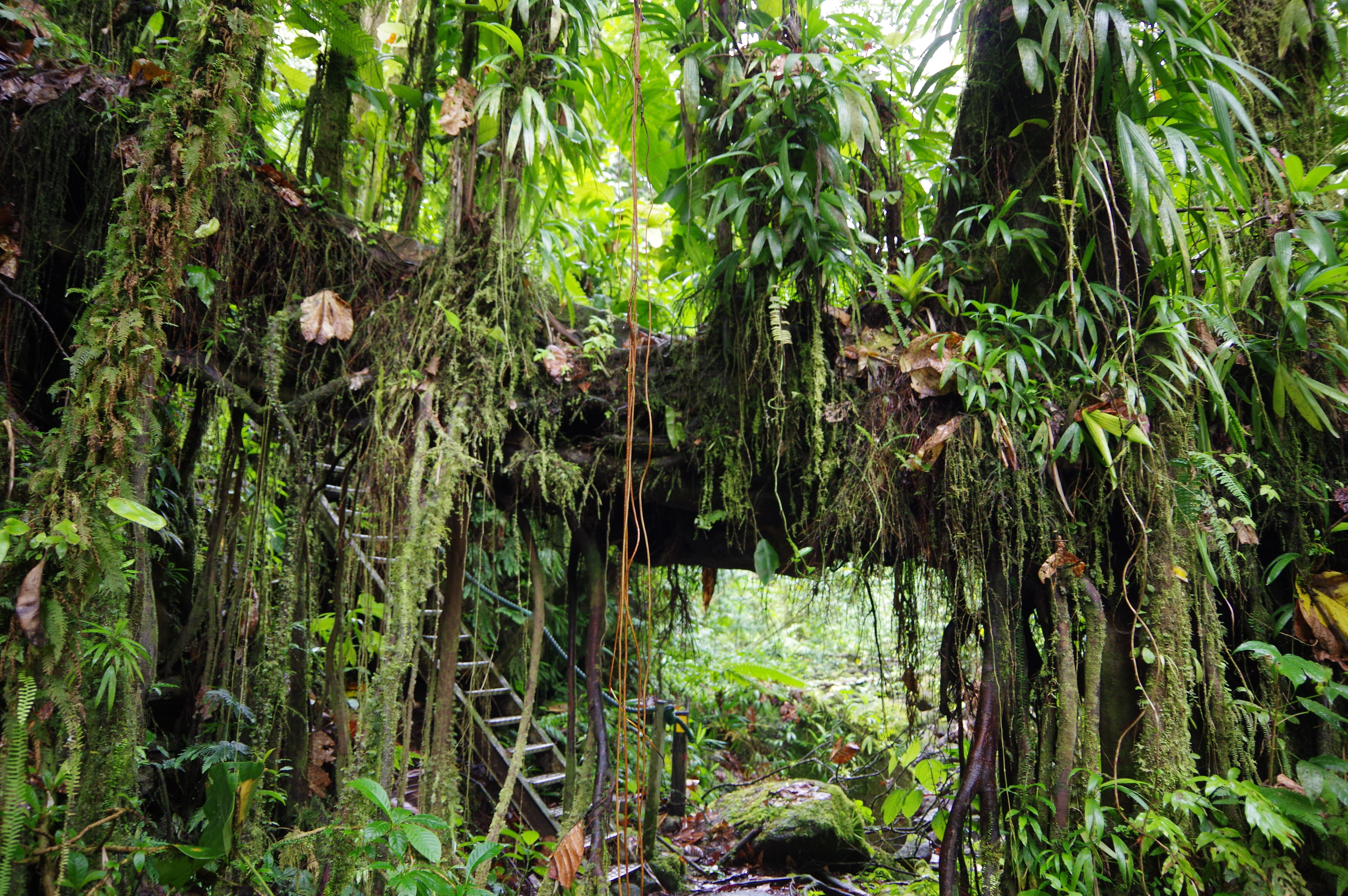 |
| Guadeloupe. Mart.wain, Wikimedia |
Ecology: These are the most diverse regions of the
planets; a single square kilometer can include trees from over 1,000 species.
Consistent rain and sunlight support dense forests, but the rain also leaches
nutrients from the soil; competition for light and nutrients amongst plant life
is fierce. So little light penetrates to ground level that, aside from tree
trunks, it’s fairly clear of vegetation. A single area of rainforest can often
be divided vertically into distinct microbiomes dominated by different species.
Climbing, jumping, gliding, and flight are common adaptations to allow travel
between trees without descending to the ground.
At higher elevations—above 500 m or so—rainforests tend to
have shorter trees and thicker undergrowth. Where the elevation is high enough
for clouds to be below canopy height, cloud forests form, with frequent
fog and extremely moist conditions that support mosses and ferns.
Conversely, at low elevation broad swamps can form along
riverbanks, with permanent or seasonal shallow water over the forest floor.
Society: Beneficial though rainforests are to
wildlife, from a human perspective they’re more hostile. Hunter-gatherer tribes
can thrive on the high productivity and moderate seasons, but to technological
societies these are barriers. Thick plant growth and extremely wet conditions
make travel difficult except by foot, and these regions still include some of
the least accessible areas on Earth. There will typically be large rivers that
make convenient avenues for travel, but these are often bordered by broad
swamps and thick vegetation that make landings difficult. Diverse diseases,
parasites, and predators are further hazards.
Of course, it’s
hard to say how much of this is inherent to rainforest climates, and how much
is a result of societies from temperate climates trying to apply technology
developed there to a new environment.
Frequent heavy rain
is a challenge for construction and sanitation, but also leaches nutrients from
the soil, making agriculture difficult, but not impossible. Inhabitants often
use “slash-and-burn” farming, clearing an area of land to farm for several
years, then leaving it to regrow while moving to a new location. While this is
sustainable in principle, growing demand for food, in combination
with logging, has led to mass deforestation.
Even when
uncultivated, the high diversity of rainforest life makes them an excellent
source of new edible fruits (including bananas, sugarcane and
possibly papayas) and medicines. They are also the original source of rubber
plants, and much is still grown there.

Tropical Monsoon (Am)
Less than 2
mm/day but more than (100 – [total annual precipitation (mm)] / 25) mm total
rain in the driest month of the year.
Examples: Southwest Indian coasts; Sierra Leone;
Miami, Florida.
Conditions: This zone can be divided into two
subtypes: Areas on the perimeters of rainforest zones that have similar wet and
dry seasons that are somewhat more pronounced; And areas affected by monsoon
wind patterns that have extremely wet summers—sometimes over 30 mm/day—and dry,
sometimes rainless winters (winter months with no rain still satisfy the
requirements if total annual rainfall is over 2,500 mm).
 |
| Varandha Ghat, India. Cj. samsom, Wikimedia |
Ecology: Those areas bordering tropical rainforest
are largely indistinguishable from them. Vertical microbiomes are less
distinct, while more pronounced wet and dry seasons may lead to seasonal
flooding. In areas caused by monsoon wind patterns, the severe dry season may
favor woodier plants and vines, but in general the intense summer rains are
sufficient to sustain thick forests.
Society: Once again, largely indistinguishable from
rainforests. Farmers do have to take the seasonal rains into account and avoid
planting crops too early before the wet season.

Tropical Savanna (Aw/As)
Less
than (100 – [total annual precipitation (mm)] / 25) mm total in the
driest month.
Examples: Serengeti; Bangkok, Thailand; Havana, Cuba.
Conditions: As with the monsoon zone, there are two
major subtypes: Regions on the perimeter of large rainforests, with moderate
wet summers and dry winters, and regions affected by monsoon wind patterns that
have very wet summers—sometimes over 10 mm/day—and dry winters. Moving poleward
from the center of the tropical band, the dry season gets progressively longer
and the wet season progressively shorter, especially on west coasts and
interiors that eventually transition to steppes and deserts.
As regions are dry in summer and wet in winter
due to rainshadow effects, but seasonal temperature variation is so low that
this has little practical impact. There is some temperature variation, though:
from around 20 °C in winter to 25 °C in summer.
.jpg) |
| Serengeti, Tanzania. Harvey Barrison, Wkimedia |
Ecology: In spite of the name, this zone is not all
open ground, and indeed it includes a large range of biomes; regions near
rainforest or monsoon zones with short dry seasons will often have similarly
lush forests. Areas with longer and more severe dry seasons will transition to deciduous
forests, that drop their leaves in the dry season to conserve water—this lets
more sunlight reach ground level, causing thicker undergrowth. These forests
have less diversity than rainforests, and individual species have wider ranges.
All life must adapt to long winter droughts. These forests are also more prone
to large fires.
Finally, the driest
areas transition to grassland, savanna (grassland with scattered trees) and
shrubland. Large grazing herbivores and their associated predators and
scavengers are common, many of them migrating long distances to avoid the dry
seasons. Wildfires are common enough that many species have specifically
adapted to survive or take advantage of them; grasses grow deep roots to allow
them to regrow after burns, and fast-moving predators hunt the animals fleeing
the flames. Water can become a rare commodity in the dry season, with life
concentrating around dwindling sources.
Society: Humans first developed in savannas, and
were in many ways shaped by the need to effectively move, scavenge, and hunt
there. Many of the last remaining hunter-gatherers still live there, though
this is largely because low rainfall makes these areas poor farmland.
Farming is still
possible, and wetter areas are used for growing tropical plants like sugar and
rubber, but the dry grassy areas lend themselves better to use as pasture land
for cattle. Maize (a.k.a. corn) may have first developed and been
cultivated in this climate zone, and some is still grown there today—though the
major centers of maize cultivation have moved to the humid continental zone. Sorghum,
cassava, sweet potatoes, and some types of yams also likely
originated here, and remain staple crops in much of the zone today.
B: Arid Climates
Annual average precipitation below ([annual average
temperature (°C)] * 20 + [280 if
>70% of precipitation are in 6 hottest months, 140 if 30-70% of
precipitation are in those months, 0 otherwise]) mm/year (definitions for the other
climate groups implicitly exclude regions with precipitation this low).

Hot Desert (Bwh)
Annual precipitation less
than half the threshold for arid climates, monthly average temperatures above 0
°C in all months (Some sources use
annual average temperature above 18 °C for the hot/cold distinction instead).
Examples: Sahara; Arabian Desert; Cairo, Egypt; Phoenix,
Arizona.
Conditions: The driest regions of the world; some
areas can go years without any rain. When rains do happen, they’re typically
brief and intense. Average temperatures are lower than equatorial rainforests,
but highly variable and so these areas have the hottest summer temperatures:
Average summer temperature is often over 30 °C and peak temperature can exceed
50 °C. But in winter average temperatures drop to around 15°, and daily
temperature ranges can exceed 20 °C—meaning that nights can drop below 0 °C, if
infrequently.
Even cloud cover is
generally uncommon, though areas near western coasts are notably cooler (closer
to 20 °C in summer) and have frequent fog due to the influence of cool ocean
currents—not that this increases precipitation much.
Sand and dunes only
cover 1/5 of global deserts (hot and dry); much of the driest areas are covered
in closely packed rocks resembling cobblestones or bare bedrock, and areas of
soil and mud exist as well.
 |
| Sahara, Libya. Luca Galuzzi, Wikimedia |
Ecology: Life is rare, but not absent. Relatively
wet areas can support shrubs, cacti, and even trees, though all tend to be
woody with small leaves. Much of the animal life burrows underground to avoid
midday heat, and all life has adapted to minimize water loss. Rare heavy rains
can cause brief growths of grass and flowers, which release seeds that will
remain dormant until the next opportunity. In regions with fog, plants
specialize to extract moisture from dew rather than rain.
But in the very
driest regions, life is largely restricted to passing migratory species.
Society: Deserts are, for the most part,
essentially uninhabitable. Barring an alternative source of water besides
rainfall, agriculture is impossible, and much of the desert is covered in
shifting sand or bare rock that couldn’t support crops even with water.
Notable exceptions
are regions with large rivers flowing in from wetter areas, such as the Nile,
Indus, or Tigris and Euphrates. Despite the lack of rain, seasonal flooding of
these rivers provides sufficient moisture and nutrients for growing crops, and
uninterrupted sun by day lends itself to very productive agriculture. Thanks to
this many of our earliest civilizations emerged in desert climates (though some
may have been slightly wetter at the time) and so desert zones ironically
included some of the most agriculturally productive areas of the ancient world.
Elsewhere, oases
fed by underground aquifers also provide small islands of habitability and goop
crop productivity. Hilly and mountainous regions can also have sheltered river
valleys, though in those areas flash flooding during heavy rains is a concern.
Away from these
water sources, permanent settlements are rare. Nevertheless, various societies
have at one time or another found it necessary to cross deserts for migration,
trading, warfare, or resource extraction. Caravans trace routes between oases
and wells, and control of these routes has often been a major strategic and
economic concern for neighboring societies. Sometimes the traders themselves
can become distinct nomadic societies.
In spite of these
connections, large deserts can be significant barriers to the spread of
societies, culture, and technology.

Cold desert (Bwk)
Annual precipitation less than half
the threshold for arid climates, average temperature below 0 °C part of the year.
Examples: Gobi Desert, Patagonia, Great Basin
Desert.
Conditions: These regions generally still have hot
(15-20 °C) summers, but freezing winters. Snow is rare but possible. Daily
temperature ranges are large just as in hot deserts, and clouds uncommon; Given
that they’re formed mostly by rainshadow effects, few deserts of this type
border the sea.
 |
| Gobi Desert, Mongolia. Doron, Wikimedia |
Ecology: Similar in most ways to hot deserts. Peripheral
areas can support grasses and shrubs, and milder summer temperatures benefit
plant life. But life here has to contend not only with hot days, but cold
nights and winter frosts as well.
Society: Because these regions are typically far
inland, they rarely have large rivers running through them and so are less
likely to feature the productive river floodplains that hot deserts do. Like hot
deserts, trade and movement across these areas is difficult but often
necessary. Just as for wildlife, milder summers are easier to contend with but
cold nights are more hazardous.

Hot steppe (Bsh)
More than half the precipitation
threshold, above 0 °C in all
months (again, some sources use 18 °C annual temperature as the hot/cold
boundary).
Examples: Sahel; Lahore, Pakistan; Monterrey, Mexico.
Conditions: Somewhat wetter than hot deserts and
bounding them on all sides. Summer temperatures and daily temperature variation
are generally lower than for deserts, but not by much. Steppes on the
equatorward side of the desert belts have relatively wet summers and dry
winters, while those on the poleward side have dry summers and wet winters like
the Mediterranean zone. There are also areas affected by monsoon winds that can
have brief, intense wet summers with rains over 5 mm/day, and rainless winters
(these aren’t well represented by this tutorial, but are small in extent).
 |
| Sahel, Mali. NOAA |
Ecology: These are, like savanna, transitional
zones; the wettest regions can have scattered deciduous forests, while the
driest are nearly as barren as deserts. The forests are only common in areas
affected by monsoon patterns, and are dominated by woody plants; in most of
this zone, grassland and shrubland dominate. Herding animals and associated
species can be common in the wet season. As in tropical savanna, wildfires are
common.
Society: Despite the low precipitation, agriculture
is possible and even quite productive on the banks of large rivers—though these
aren’t as vital as for deserts. Some varieties of millet may first have
been cultivated here. Pastureland can also be productive here. Unlike most
desert areas, agricultural productivity is high enough and access to water easy
enough that widespread settlement is possible even far from major water
sources.

Cold steppe (Bsk)
More than half the precipitation
threshold, below 0 °C part of the
year.
Examples: Central Turkey; Central Spain; Denver,
Colorado.
Conditions: These regions have more consistent
moderate precipitation throughout the year than hot steppes, and subfreezing
winter temperatures, so they do usually have some snow in winter. Outside of
the Hadley cell, precipitation more often comes in the form of distinct storms
than daily rain. Some of these regions appear in highlands as a transition from
wetter lowland climates to dry mountain plateaus.
 |
| Badlands National Park, South Dakota. Wing-Chi Poon, Wikimedia |
Ecology: Again, these are mostly grasslands and
shrublands, and include American prairies. Mild summers makes evaporation
slower than in hot steppes and these areas are generally more hospitable to
life without adaptations for hot and dry conditions. Large herding animals and
small burrowing animals are common.
Society: This is the arid zone most hospitable to
widespread settlement. Productive agriculture is possible even far from major
rivers, and potatoes may have originated in highland areas of this zone.
Dryer areas are still more often pastureland. Population density is generally
low, but large cities are more common than in deserts or hot steppes.
C: Temperate Climates
Coldest month between 0 °C and 18 °C, hottest month above 10 °C (some sources use -3 °C in the
coldest month as the temperate/continental distinction instead).

Mediterranean (Csa/Csb/Csc)
3 times more rain in the wettest month of
winter than the driest month of summer, driest month in summer below 1 mm/day.
Examples: Coastal Mediterranean (big surprise); US
west coast; Cape Town, South Africa; Santiago, Chile.
Conditions: In many ways a transition between arid
steppes and more humid temperate climates, and somewhat unusual in having
significantly wetter winters than summers due to the alternating influence of
the horse latitudes and the polar front. More equatorward regions (Csa)
resemble steppes in many ways: hot summers (25 °C ) with high temperature variability (10 °C), and low rains even in the wet
season (<3 mm/day). Further poleward or at higher altitude (Csb/Csc),
temperatures are more moderate and winter rains can exceed 5 mm/day, with
occasional snowfall. Where these regions lie on the coasts of major oceans,
cold currents cause frequent morning fog.
Rarely does this climate zone reach far from the coast; it’s
only because of the particular position and geography of the Mediterranean sea
on Earth (And the southwest coast of Hutton on Teacup Ae) that it covers so
much area. A notable exception is in highlands in the tropical or desert belts,
where seasonal rainshadows can create the requisite dry summer/wet winter
cycle.
.JPG) |
| Peñón de Alhucemas, Spain. Kokopelado, Wikimedia |
Ecology: Though small in extent, the life in these
regions is very distinct. Hot, dry summers favors life adapted for steppes, but
high average precipitation and mild temperatures favors life from other
temperate zones. Much of the zone has a “mosaic” landscape, with small areas of
forest, savanna, shrubland, and grassland mixed together. Small variations in
access to water in summer can be very impactful; wooded streambanks often exist
in close proximity to grassy hilltops. Evergreen, deciduous, and coniferous
trees are all mixed as well, though with some division by latitude and altitude.
Equatorward, low-altitude mosaic landscape gives way to poleward, high-altitude
pine forests.
Animal life is similarly a mix of groups also seen in
tropical and temperature climates. This zone tends to lack the large migratory
herding animals more common in steppe zones, but do retain the small burrowing
animals. Cold-blooded animals that can’t withstand cooler poleward winters are
common here.
Despite the broad milieu, most life has some adaptation to
the dry summer conditions, as well as the frequent wildfires. Small shifts in
average rainfall can dramatically increase the proclivity to fierce fires in
forest areas.
Society: Though civilization didn’t begin here, many
early large societies did develop in the Mediterranean zone—though only in the
areas around the eponymous sea. It’s a bit early in this series to speculate on
exactly why, but perhaps a mix of very mild winters and wet enough conditions
for easy agriculture can be credited. Today this zone is widely regarded as
among the most comfortable regions, and tourism is popular.
Wheat, barley, and rye all likely originated
in this zone, and possibly oat as well; the short wet seasons and long, hot
dry seasons seem to lend themselves to the development of plants that grow
quickly and produce durable, easily stored seeds. Olives and grapes
are also widely grown, and wine and beer were likely first
developed here. These are not the most productive regions today but are known
for the wide diversity of foodstuffs they produce.

Humid Subtropical (Cfa/Cwa)
Hottest
month above 22 °C, above 1 mm/day
average precipitation in all months of summer.
Examples: Southwest China; Southwest USA; Milan,
Italy; Johannesburg, South Africa.
Conditions: As the name implies, these are wet
regions, in some cases comparable to rainforests in summer (>6 mm/day) but
also including more moderate regions (3 mm/day). The major distinction is
between the main (Cfa) regions with consistent rains throughout
the year, and monsoon-infuenced (Cwa) regions with 10
times more rain in their wettest month than their driest month. The former
dominates in the main areas at mid latitude on eastern coasts, while the latter
appears in highlands and areas with monsoon wind patterns.
Summers are, by
definition, quite hot, and rarely do winters drop below freezing. Thunderstorms
are common, and these areas are often the most prone to hurricanes and
tornadoes.
 |
| Bayou Corne, Louisiana. jc.winkler, Wikimedia |
Ecology: Much of this zone is dominated by dense
forests of evergreen plants, especially close to the border with the tropical
band. Density of vegetation can be comparable to tropical rainforest, with
fierce competition for sunlight and canopies blocking most sunlight, though
vertical microbiomes aren’t as distinct. These regions are so moist that many
plants have to adapt to shed water rather than retain it. On flat ground,
swamps are common on coastlines and along rivers.
More poleward, less
packed forests predominate and there are more areas of open ground. In the
driest areas forest can give way to grassland, though these are less extensive
than for the Mediterranean zone.
Society: To some extent the more equatorward areas
present much of the same hazards as tropical rainforests: dense plant growth,
heavy rains, risk of disease, etc. But temperatures are milder and soil quality
is notably better; some of the earliest agriculture began here, and these
remain among the most productive farming regions in the world. Rice and soybeans
originated in this zone and are still mostly grown here today.

Oceanic (Cfb/Cfc/Cwb/Cwc)
Hottest month below 22 °C, above 1 mm/day
precipitation in summer.
Examples: British Isles; North and central France;
New Zealand; Vancouver, British Columbia.
Conditions: This is probably what leaps to mind when
most people imagine a “temperate climate”, with mild temperatures, consistent
rains, and strong but not extreme seasons. The major subtypes, from most
equatorward to most poleward are subtropical highland (Cwb),
which appears in highland regions in the tropics and so has consistent average
temperatures across the year (15-20 °C) but high daily temperature ranges (15
°C), and very distinct wet summers (5 mm/day) and dry winters (<1 mm/day); marine
(Cfb), the dominant form at mid latitudes, with mild summers
(15-20 °C) and winters (5-10 °C), consistent rains throughout the year (2-5
mm/day), and occasional but not persistent frost and snow; and subpolar
(Cfc/Cwc), in small areas in mid-latitude highlands and
high-latitude coasts, which are broadly similar to marine but 5-10 °C cooler
throughout the year, with winter nights regularly below freezing.
 |
| Moor, England. dennisredfield, Wikimedia |
Ecology: This zone is predominantly forest, with a
mix of evergreen, deciduous, and coniferous trees. Trees are lower and the
canopy less packed, so there’s more undergrowth here than in more equatorward
forests. Some of the wettest areas on the coasts feature temperate
rainforests, with consistent intense rains and high canopies.
Large herbivores
and predators are fairly rare. Average temperatures are low enough that
cold-blooded species are also rarer than in other temperate zones, with small-
and medium-sized warm-blooded forest animals dominating.
This zone also
includes many montane forests and grasslands at lower latitudes, which
have an unusual combination of low temperatures and intense sunlight. At lower
altitudes these regions include some of the cloud forests mentioned earlier,
while at higher latitudes they give way to shrubs with waxy surfaces to retain
moisture. High winds and little available soil become a major obstacle, and so
plants tend to be low and slow-growing.
Society: Agriculture and dense cities were slow to
arrive in these areas, but in more recent times this region has hosted major
centers of industry and urbanization. Neither summers nor winter are harsh,
agriculture is reliable, and there are no major terrain hazards; dense forests
and swamps can create some geographic barriers but not to the same extent as
rainforests in warmer climates. Harsh winter blizzards and frosts are not the
norm, but frequent enough to be a hazard to life here without proper shelter.
D: Continental Climates
Coldest month below
0 °C, hottest month above 10 °C.

Humid Continental (Dsa/Dsb/Dwa/Dwb/Dfa/Dfb)
At least 4 months above 10 °C.
Examples: Poland; Northeast USA; Seoul, South Korea;
Moscow, Russia.
Conditions: In many ways this climate resembles the
temperate zones, but with 3-5 months with subfreezing temperatures. The
subtypes are hotter (Dsa/Dwa/Dfa) and cooler (Dsb/Dwb/Dfb)
areas with precipitation patterns resembling those of mediterranean (Dsa/Dsb),
monsoon-influenced humid subtropical (Dwa/Dwb), and marine
oceanic (Dfa/Dfb) patterns, though precipitation patterns
are overall less impactful here to life and society.
Heavy winter snows
are common, and oscillations in the position of the polar front in winter tends
to cause cycles of milder and colder periods.
 |
| Table Mountains, Poland. Poconaco, Wikimedia |
Ecology: This is a very broad region, encompassing
dense forests, broad grasslands and prairies, and highland shrubs. The unifying
element is the strong seasonality; long, hot summers provide plenty of time for
growth, but all species need some adaptations for the subfreezing winters.
Trees are predominantly deciduous—shedding vulnerable leaves in winter—or
coniferous—with smaller, tougher leaves such that they can be retained
year-round. Many animals either migrate, leaving for warmer climates in winter,
or hibernate, minimizing energy consumption.
Cold-blooded
animals are not absent but uncommon and small, and many animals have some
insulating fur or feathers to protect from the cold—sometimes with alternating
long and short coats that are grown and shed with the seasons. In some of the
more open areas, herds of migrating herbivores and their associated large
predators and scavengers are common, somewhat akin to those in tropical savanna
despite the vastly different climate conditions.
Society: Though agriculture was slow to come to
this zone (excepting perhaps some highland areas in the near east) it now
includes some of the most agriculturally productive areas in the world. Some
varieties of East Asian millet likely originated here. Much of the
world’s lumber production also occurs in this zone.
Strong seasonality
is the hallmark of this zone. Warm summers bring good growing seasons, but the
harsh winters are a consistent challenge. Spring and fall also tend to be
accompanied with “mud seasons”, when heavy rains or snow melt combined with
little sunlight and cool temperatures causes large amounts of standing water
and mud to cover much of the ground. Travel in these times is difficult in
areas without paved roads.

Subarctic (Dsc/Dsd/Dwc/Dwd/Dfc/Dfd)
No more than 3 months above 10 °C.
Examples: Central Finland; Siberia; Anchorage,
Alaska.
Conditions: Shares essentially all of the same
subtypes as humid subcontinental, but they’re even less impactful here. Summers
are usually around 15 °C, but winters can plunge below -30 °C, and much of this
zone spends more time below freezing than above it. For the most part
precipitation is lower than in temperate zones, but not as low as steppes.
 |
| Alaska Range, Alaska. NOAA |
Ecology: This zone is dominated by taiga,
A.K.A. boreal forest, vast stretches of forest dominated by a relatively
small number of mostly coniferous trees; biodiversity is much lower here than
in warmer forests. Summers may be short, but the days are long, and much of the
life here is adapted to take advantage of the sun even in cold conditions.
Though rainfall is low, slow evaporation and melting snow make for moist
conditions, so moss and lichen are common.
There is little
biological activity in winter; plant life falls dormant, and animal life either
migrates away or hibernates.
Society: Agriculture here is possible, but fairly
unproductive. Hunting, trapping, and fishing are more reliable sources of food
in many areas, and lumber and fur production are major industries. Population
density is generally fairly low and infrastructure undeveloped. These are
marginal areas, with most activity concentrated on survival rather than, say,
empire-building.
E: Polar and Alpine Climates
All months below 10
°C.

Tundra (ET)
Hottest month above 0 °C.
Examples: Coastal Greenland; Central Himalayas;
Central Alps.
Conditions: Brief summers and long, cold winters often
plunging to below -50 °C. Precipitation is generally low, even lower than steppes
and deserts in warmer areas, though low temperature means that evaporation is
slow so this has little bearing on surface conditions. Snow covers the ground
through much of the year, but does melt in summer.
Most of these areas
are around the periphery of the ice caps, but they also occur in high, isolated
mountain plateaus, even close to the equator, and these areas have milder
winters.
 |
| Sydkap, Greenland. Hannes Grobe, Wikimedia |
Ecology: Some taiga reaches into this zone, but for
the most part it’s a barren environment limited to grasses, shrubs, mosses, and
lichen. This is due not only to low surface temperature, but permanently frozen
soil less than a meter below the surface. Some large grazers and predators can pass
through in summer. Almost all life is warm-blooded.
The seas are far
more productive, and so some of the coastal areas are populated by amphibious
or flying predators, and some predators and scavengers preying on them.
Society: As with animal life, most human life in
these areas are dependent on the sea, so settlement is largely limited to
coastal fishing villages. In inland areas, some settlements can survive on
hunting or raising livestock that can feed on the limited grasses and shrubs.

Ice Cap (EF)
All months below 0 °C.
Examples: Antarctica; Central Greenland; Mount
Everest.
Conditions: As you’d imagine, this area is
permanently covered in ice; often large, thick glaciers. Average temperatures
in the interior are often below -30 °C,
and precipitation is comparable to deserts. Some isolated valleys can remain
ice-free due to many years with no snow.
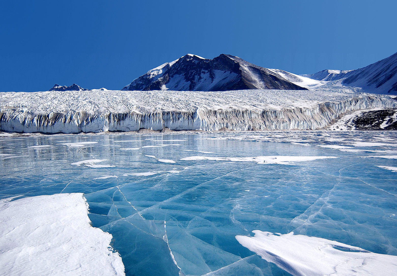 |
| Lake Fryxell, Antarctica. National Science Foundation |
Ecology: Little life to speak of. Plant growth is
impossible, so for the most part the only source of food is the sea. The inland
areas are populated solely by passing amphibious or flying predators, and some
marginal microbes.
Society: Again, not much. There are no permanent
settlements here save for research stations, which have to be supplied from
elsewhere. Harsh winter storms and glacier crevices are extreme hazards.
Biomes and Biogeographic Regions
As I mentioned near the start—and as should have become
clear in the last section—the climate zones don’t perfectly predict the biomes
of a world. Development of distinct biomes depends on factors like evaporation,
soil quality, and water supplies other than precipitation. There are some
alternative climate zone systems, like the Holdridge system,
that better account for these factors, but require more precise data or
calculations that are impractical to do by hand.
 |
| One breakdown of Earth's biomes. Ville Kroistinen, Wikimedia |
Still, the differences aren’t too great, and having a little
authorial freedom to determine the precise biome types isn’t exactly the worst
burden. I think I’m comfortable settling for the Köppen system as a template
for Teacup Ae’s climate.
But one other factor we can determine now is the breakdown
of biogeographic regions. These are, in a sense, the ecological equivalent of
continents: large areas divided by barriers like deserts, mountains, or seas,
or by the sharp transition between temperature and tropical climates, and each
represents an area within which successful types of land animals or plants can
circulate on short evolutionary timescales; put another way, different regions
with the same climate may have similarly structured ecosystems, but will have
different groups occupying the same niches.
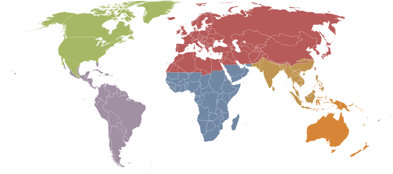 |
| Earth's major biogeographic regions (save for Oceania and Antarctica). carol, Wikimedia |
To mark them out, group together clusters of continents and
islands, and divide them roughly along the desert belt or the tropical-temperate
boundary, save for in cases where the tropical or temperate areas of that
cluster are too small to have much diversity of their own. Regarding islands,
try to take geological history in mind; areas recently split from the mainland
are likely to still have similar life, and may still have shallow waters
separating them or may become connected again in times of low sea level.
That in mind, here’s how I’ve broken down Ae, along with
some names for the biogeographic regions for later reference. When we think
about wildlife in a later post, this will help give us an idea for how to
distribute them.

In Summary
- Climate zones can be classified based on temperature and precipitation patterns across the seasons.
- The atmospheric convection cells and associated prevailing winds cause major climate bands:
- Rainforest near the equator.
- Deserts near the horse latitudes, except on eastern coasts.
- Temperate at mid latitudes.
- Tundra and ice caps near the poles.
- Large mountain ranges can cause high rains on their windward sides and dry rainshadows on their leeward sides.
- Ocean currents bring warm waters to western coasts at high latitudes and cool waters to eastern coasts at high latitudes and western coasts at low latitudes.
- High mountains have climates more typical of higher latitudes (by about 8° latitude per km elevation).
- Oceans form ice sheets when they drop below -2 °C
- The ITCZ and other convection cell boundaries move with the seasons, causing monsoon rains and similar patterns.
- Prevailing winds are caused by a combination of the atmospheric convection cells and local pressure zones caused by surface temperature.
- Winds carry moisture inland from the coasts, causing precipitation thaat generally decreases further inland, save for where it is increased by converging winds and orographic rains.
- Köppen climate zones are defined by temperature and precipitation patterns across the seasons: (notes: Temperature values are averages for the months of peak summer and peak winter; precipitation averages are rough guidelines; for all zones except Mediterranean, summer is presumed to be the wettest season).
Climate Zone
|
Temperature
(°C)
|
Precipitation
(mm/day)
|
||||||
Summer Min
|
Summer Max
|
Winter Min
|
Winter Max
|
Summer Min
|
Summer Max
|
Winter Min
|
Winter Max
|
|
Group A
|
18
|
Wet
|
||||||
Rainforest
|
18
|
Very Wet
|
Wet
|
|||||
Monsoon
|
18
|
Wet
|
Wet
|
|||||
Savannah
|
18
|
Wet | Dry | |||||
Group B
|
Dry
|
Dry
|
||||||
Hot
Desert
|
0
|
Dry |
Dry
|
|||||
Cold Desert
|
0
|
Dry |
Dry
|
|||||
Hot
Steppe
|
0
|
Dry (border) |
Dry
|
|||||
Cold
Steppe
|
0
|
Dry (border) |
Dry
|
|||||
Group C
|
10
|
0
|
18
|
|||||
Med.
|
10
|
0
|
18
|
Dry
|
Wet
|
|||
Subtropical
|
22
|
0
|
18
|
Wet
|
||||
Oceanic
|
10
|
22
|
0
|
18
|
Wet
|
|||
Group D
|
10
|
0
|
Wet
|
|||||
Humid
Continental
|
10 (>3 months)
|
0
|
Wet
|
|||||
Subarctic
|
10 (1-3 months)
|
0
|
Wet
|
|||||
Group E
|
10
|
|||||||
Tundra
|
0
|
10
|
||||||
Ice Cap
|
0
|
|||||||
Notes
In case anyone wants them, here’s a group of maps of each of
the individual Köppen climate zones on Earth (along with some regional maps). Note
that some depict current zones, and some show near-future predictions of how
zones will move as global climate warms.
Should someone want to follow me down the rabbit hole of
trying to find a reasonably usable GCM, here are my findings:
- ROCKE3D is probably the most promising, with good documentation and intentional design for flexibility and use with exoplanets, but 1, I’m not confident it will run well on home computers, and 2, there’s little explanation of how to import novel topography into the program other than to note that it’s hard. I’ll try running some tests with this one in the near future.
- EdGCM is by far the easiest to use, but the least customizable, and again there’s no clear way to add topography—but it would probably be similar to the process for ROCKE3D, given their “shared ancestry”.
- FOAM has a pretty clear process for importing topography, but the program itself doesn’t appear to be publicly available.
- PlaSim has a basic and awkward topography editor, and isn’t too hard to get working (if you’re willing to install linux), but for the life of me I can’t figure out how to interpret the output.
- MitGCM is one I’ve seen a few worldbuilding sites recommend, but I’ve never seen anyone claim to have actually used it.

.jpg)
.JPG)
For climate bands, how do you determine winter and summer with the thermal equator since winter/summer isn't perfectly down the middle. I'm not sure if I'm just reading the tropical zone on Lyell wrong, but I'd think there'd be another temperate section in the middle based on winter in the southern hemisphere
ReplyDeleteFor the climate bands, which you're drawing based on temperature, summer and winter are defined as the hottest and coldest months, regardless of hemisphere; so for drawing the temperate band, anywhere that drops under 18 C at any point would be excluded, regardless of when in the year that happens. For the climate zones within the bands, which you're drawing based on precipitation, summer and winter are formally defined as the months with most and least sunlight; where seasons are mostly obliquity-driven such as here, you can divide the planet by the equator and assume opposite seasons in opposite hemispheres; where seasons are mostly eccentricity-driven, you'll have global seasons that are the same across hemispheres.
DeleteHi, great series you've done so far, it's been a massive amount of help with the current project I'm working on. Though there is one thing I'm stuck on, my planet has an obliquity of about 72 degrees, meaning that it effectively does not have an ITCZ or thermal 'equator' and I have a feeling this would effect ocean climates too. I guess it also doesn't help that the planet has a rotation of 16 hours but I'll ignore that for now.
ReplyDeleteHow would one sort out such extreme scenarios like this? Massive thanks in advance if you get the chance to respond, otherwise stay safe!
Yeah, high obliquity is basically a whole other ball game. You can even end up with totally flipped convection cells, and winds converging at the poles rather than the equator. If you look back at the last post, Part VIa, I discussed some of the broad climate patterns we'd expect with high obliquity. Next post I'll try to actually chart out climate zones of a world with 90 degrees obliquity and an ice belt, but frankly it's going to be a lot of guesswork.
DeleteThanks! Can't wait for the next post.
DeleteIt's not my area of expertise but I too have been looking for a GCM that could be used for world building. The inability to find one has almost motivated me to try to write a (very simple) one from scratch. It would only have to produce plausible rather than completely accurate results for varying inputs. However, that's more work than I have spare time for right now. I did see Exeter University's ISCA referenced in some papers but I haven't had chance to grab it from Github and give it a go. Documentation is sadly rather minimal at present though.
ReplyDeleteI have actually been contacted by someone who's managed to get ROCKE-3D working at home. From what they tell me it is possible to get running on a laptop, though it's not easy--takes a good amount of time learning the setup process, and you may need to work up some custom scripts for importing topography--and if you left it to run overnight for around 8 hours every night, it would probably take months to complete. I also just stumbled across OASIS, which looks promising (https://software-oasis.com/), but it doesn't appear ready for public use yet.
DeleteI must admit that the significant processing time required sometimes makes me think that perhaps a GCM may not be the best approach anyway. A "simple" 2D energy balance model might be better though the ocean, atmosphere and a water balance model would need to be added in some way. I suspect no tool that anyone else produces would be sufficiently flexible for me as I want the ability to arbitrarily define the spatial distribution of irradiance to cover all possibilities. For example, binary star systems, spin-orbit resonance, exomoons, reflective gas giants, etc. The method in this paper (https://arxiv.org/abs/1906.05844) at least provides details on an energy balance model though unfortunately it says nothing about precipitation and wind. Is it really too difficult or incorrect to add a simple parametric approximation somehow though?
DeleteROCKE-3D is designed for flexibility--it can certainly handle spin-orbit resonances, and I'm not sure how it handle multiple stars, but for a distant-orbiting S-type planet you can probably get a good enough model by taking the spectrum of a star and doubling the luminosity (as to exomoons, my reading so far indicates that eclipses and reflected light should almost never have a significant impact on climate). Still, the time required is very daunting.
DeleteBut as to the energy balance model, that is more-or-less what Clima-Sim is, and it works reasonably well for fairly Earthlike cases but simply can't produce reasonable results for high eccentricity, high obliquity, or tidal-locked worlds. I can't say if that's a particular problem with the model assuming Earthlike patterns of heat flow, or a more essential problem with the ability for a model of this type to represent the more vigorous patterns of circulation on these worlds. It also doesn't provide any info on winds or precipitation patterns, though it must necessarily be modelling air circulation to some extent, and it does seem to at least partially model latitudinal cloud cover. Given how much GCMs seem to diverge in predicting precipitation in formal research, I fear there may just be a minimal level of simulation complexity required to produce consistent and reasonably accurate results.
At work I've recently been looking at NVIDIA's new tool called Modulus for developing physics machine learning models that can be used for electromagnetic modelling. However, it can also theoretically be used for climate modelling and in fact NVIDIA did just issue a press release saying it would be used to produce a digital twin of Earth to help climate science. I wonder whether a basic climate model using GPU acceleration could be implemented to help worldbuilding.
DeleteApparently OASIS https://software-oasis.com/oasis/ is intended to be GPU-accelerated, but there doesn't seem to be a publicly available version yet.
DeleteThanks for the guide! it was very useful. I have just a question though, my world has a slower spin and it has the high pressure bands at 45º N/S and the polar low pressure bands at 70º N/S. What would it mean for the location of the high pressure spots and the fronts?
ReplyDeletePush the anticyclones further poleward, which will maybe give you long and high-angled (but perhaps weaker) fronts, and reduce the area affected by the polar front. Desert bands will be further poleward of course, but the ITCZ may actually wander more with the seasons so it might be a bit less distinct. If you go to the next section you can see I tried to sketch out climate for a slower-spinning world--though much slower than for you, I'm guessing.
DeleteYeah, my world takes more or less 64h to spin, so there are three circulation cells, though the temperate and polar cell are a bit squashed by the hadley cell. One factor that made me have some issues with the winds and all is that the world´s landmasses are very fragmented by tidal stresses from its parent planet and strong tectonic activity, added to the world being relatively young (3.5 Gya) it leads to 16% continents and lots, LOTS of shallow seas . My largest continent is about the size of the Sahara desert, so I don´t know if it´s big enough for any big pressure system
DeleteI'd say that's still big enough, and small seas between landmasses may "count" less than open oceans, in the same way that the Mediterranean and the Caspian don't provide as much moisture to the surrounding landmasses as the Atlantic does. But you may very well just end up with no substantial deserts, and instead just a few dryish rainshadowed spots.
DeleteI was going through your guide and climasim, but since I had a map that had much higher detail than yours I chose to use climasims at sea level output and manually adjust temperature for altitude, with -4.46 C for every km because that's what climasim does (?). But in other locations I found that the lapse rate is actually 6.5 C/km (according to aviation) on average.
ReplyDeleteAny thoughts/advise on how I should approach this?
This is actually addressed by the clima-sim author (if you click on the blue bits of text in the program, there are helpful popups explaining some of the underlying logic). 6.5 C/km is accurate for open air, but for large highland areas the rate is lower because of heating of the land surface by the sun. So use the lower rate for large plateaus and mountain ranges, and the higher rate for more isolated peaks.
DeleteWhat happens when the ITCZ is directly over a subtropical high or completely crosses it?
ReplyDeleteThat shouldn't be possible. The ITCZ is necessarily a low-pressure zone, and however far it moves with the seasons, the highs should move farther to keep well clear of it.
DeleteOh, so does that mean the subtropical highs could move as far north as 60° and over land to keep away from the ITCZ?
DeleteIf there's an ocean that the ITCZ completely moves past, the high in that sea may just disappear in summer. Generally speaking, though, the model I'm presenting here gets a bit iffy when you don't have large ocean basins across all latitudes, as well as for cases with that much ITCZ movement. The thing to remember here is I'm trying to take Earth's atmospheric regime and stretching it to fit other, similar worlds, but there will be some thresholds past which those worlds just switch into a different regime--and right now, we don't really have the data to say exactly where those thresholds will be.
DeleteThis is amazing, someone should award you with an honorate degrees in all the sciences. One question though: Considering Climasims only runs on Windows, has anyone found an alternative for Mac? Thanks in advance!
ReplyDeleteSo far as I'm aware, no, it's a somewhat obscure bit of software. If it helps, I'm working on a tutorial for a more advanced piece of software (exoplasim) that's a good deal more effort to get working but may actually work on Mac. I'm not sure though, I don't know anyone who's tried; I've had to set it up on a linux partition.
DeleteThanks for the quick answer, though I was hoping for a different one ;) I'm no computer pro so I haven't even tried to dabble with Linux (what's more, all computers I "own" are company issued, so I'd rather not set up any partitions). Do you know of a method to "manually" figure out temperature zones like Climasims does, or am I reduced to following the Artifexian method and just broadly sketch in a handful of climate zones hoping for the best? Thanks again!
DeleteThere are some more detailed tutorials on Cartographer's Guild that you could try to adapt, such as here and in the other threads linked https://www.cartographersguild.com/showthread.php?t=27782 . It is all a tad loose, but that's the best we can do by hand.
DeleteThanks a lot! I'll check that out. I'm still on the fence whether I need to go that much into detail (considering I'm worldbuilding for writing, and most readers don't care whether climates & biomes on continents that aren't even in the story they're reading make scientifically accurate sense; or whether the description of some random stretch of land features a tree that, climate-wise, should only grow 2° latitudes farther south) but I'm loving the process so far. By the way, this is a great blog. I'm amazed by your level of scientific understanding, your ability to break down the hard stuff into palatable chunks and also your willingness to tunnel into the nerdy stuff. I'll be sure to follow along while I'm working on my world, can't wait to see what you cook up next.
DeleteHi! This is such a fantastic worldbuilding guide and I've really learned a lot as well as had a blast doing it following along in the steps!
ReplyDeleteI just had a small question regarding building the tropical climate zones if that's alright? It's about this part:
"We’ll start out by marking out areas that are very wet in both seasons as tropical rainforest (Af), areas that are wet in both seasons as tropical monsoon (Am), and areas that are wet in one season and dry in the other as tropical savanna (Aw/As)."
And more specifically this part:
"... and areas that are wet in one season and dry in the other as tropical savanna (Aw/As)."
Now it might just be that I'm not understanding it right because I'm not a native English speaker, but would this not entail all remaining land that is not covered by the two preceding climate zones? Meaning areas that are Very Wet both seasons (Af) and Wet both seasons (Am) respectively that is?
The key point here is that, in the tropical band, we're distinguishing between very wet and wet areas. So if you mark in those areas as instructed, you'll be left with some areas that are very wet in one season and either wet or dry in the other season, which you then mark in as rainforest, monsoon, and savanna as instructed a little after that.
DeleteThis somewhat awkward and imprecise approach is to account for the facts that A, while the temperate and continental regions basically only have 4 levels of wetness (oceanic/subtropical zones that are wet year-round or only dry in winter, mediterranean zones that are wet in summer, steppe that's dryish year-round, and desert that's very dry year-round), tropical regions have 5 levels (rainforest, monsoon, savanna, steppe, and desert); and B, monsoon zones can either be areas that are moderately wet year-round, or those that are very wet in ones season and very dry in the other.
I see. I think I understand, I just got hyperfocused on one step (and the map shown in that step) when I should've kept going. I think I understand how to proceed now. Thank you!
DeleteGreat guide. The part I'm currently getting stuck at is the adjustments to the isotherms. The adjustment made by currents I can understand, but the adjustments based on mountains is where I'm getting hung up on. I'm trying to understand what you did, but am failing, and I believe it's because it's the part where you're altering the isotherms the most, while it is the least explained part of the tutorial.
ReplyDeleteSo basically, we expect that temperature should fall with altitude by something like 5 degrees C / km; if you have a 4-km-high mountain next to a low plain, you should expect it to be something like 20 C colder on its peak than the plains. Clima-sim will try to account for that in building the isotherms (if you have it set to), but the trouble is the low resolution of the topography: Near the equator, each cell of that grid it uses is over 1,000 km across (for an Earth-size planet). It also only has a few different elevation levels, the highest at 4000 m. So if, say, you have a ridge near the equator that's only 100 km across and 6 km high, you might input it in clima-sim in such a way that it simulates it as 1000 km across and 4 km high. The isotherms it outputs will thus show this large cold area that's much too broad, because it thinks that's how big the mountain is. So in that final adjustment step, we try to thin down that cold area to the actual size of the mountain range, and maybe cool the peaks a bit more to account for their greater height than simulated.
DeleteOh hey just fyi I noticed a typo where you put east instead of west on the equatorial currents when describing them curving back from the equatorial countercurrent. There's a diagram, so it doesn't seem like a huge thing, but I know you care about precise wording, so I figured I'd mention it rather than keep it to myself. Love your blog by the way, I've used it for a few worlds now and I always appreciate your balance of thoroughness and accessibility
ReplyDeleteHello, i have read your guide and got most of it clear, but got stuck (and probably will got more in the future) while doing it.
ReplyDeleteIm trying to make a pangea map, so guessing how far is 1000 to 3000 km is important for the inner deserts, any tip on it or is just guessing work?
It would pretty much just come down to knowing the general scale of your map or using something like gplates, which has a distance-measuring tool and can import any equirectangular map as a raster
DeleteThis comment has been removed by the author.
Deletemaking a more in depth comment.
DeleteI do have both a scale and gplates, but:
i cant have a meassure visible in gplates while using the dot tool, not that matters much to move it a bit but i prefer to avoid if possible.
and even if i could make it work that would give me a point and not an area, i could repeat it a lot to obtain the area, but thats exactly what im trying to avoid to do (repeat the point guessing like 100 times) and why i asked if there was a tip or another way to do it.
Im guessing is not possible from your comment but wanna be sure
I don't have a better idea for measuring distances quickly, no, but these guidelines are not meant to be very precise, so I really wouldn't worry about making so many measurements; for making the maps above I only referred to gplates distances maybe a handful of time to give me a general idea of the high-latitude distances.
Deletewelp time to guess a lot then.
Deletethank you a lot for your time answering me
I just want to thank you. Artifexian pointed me here, and I've already started reworking all of this into a single document and set of checklists so that I a) remember it all, b) don't need to be online and jump post to post to freshen my memory, and c) I can change things if I find a better methodology for anything or add things you don't cover. When (if) I ever get that done, all credit to you, and I'll share.
ReplyDeleteThis is a truly fantastic effort you've made.
are there other ways to do the temperature without Clima-sim
ReplyDeleteIn terms of software, there's a few other 2-dimensional energy balance models in the scientific literature if you search around, but all are going to be significantly more difficult to install and use. There's also exoplasim, which is a proper climate model, and I've written up a full installation guide in the part VI supplement, but again it's a somewhat difficult and not always fully reliable process.
DeleteThere are also some old guides on the cartographer's guild forums where people tried to work out koppen climate maps without any simulation software.
So.... im back with more doubts. :)
ReplyDeletefinally was able to do all the rain part and red through the biomes part
in deserts how should i do it? paint all the arid zone as desert and then add around a strip of steppe, or should i do it all inside the arid zone? also im guessing that shallow inclinations can be simplified as flat terrain, not sure if it has a basis or not.
on the tropical zone. is there any average distance from wich monsoon transforms into savannah?
i think that is all the doubts that i have right now before actually doing it, thanks in advance for the answers
As I recall I placed steppe inside the arid areas rather than around them. And yes, I referred to "relief" specifically in terms of a steep change in elevation; something like the gradual slope of the American midwest doesn't cause any rainshadowing effect (it does get more arid to the west there, but mostly just due to distance from the ocean).
DeleteFor the tropical monsoon/savanna zones, it's pretty variable, but looking at Earth's map, it's kind of similar to steppes, generally a couple hundred km
thank you a lot again
DeleteI tried this method multiple times for the world I'm building, and I keep encountering a few problems. Specifically, my continental zone is tiny, the majority of my temperate zone is subtropical, even on west coasts, and I have no permanent ice caps on land or sea, and my north pole doesn't even have seasonal ice. My world is fairly standard, though it is a bit hotter than earth, so is all of this expected, or did I mess something up?
ReplyDeleteHow much hotter, because yeah that all sounds like what a substantially warmer planet should look like, e.g. https://worldbuildingpasta.blogspot.com/2022/05/climate-explorations-temperature.html#30c
DeleteKind of a dumb question but how do I copy the output of the Clima-Sim formatter with out it placing tabs everywhere? I remember doing it before but I forgot how I did it.
ReplyDeleteA supercontinence
ReplyDeleteI resized the map for Clima-Sim to 720x420 pixels like you said, but it's too small and doesn't fill up the full map, is there something I'm missing?
ReplyDeleteUpdate: I resized it to 901x526 pixels and it's fitting properly now
DeleteIf a terraformed low-gravity planet had been given a massive enough atmosphere to completely counteract it and have Earthlike air pressure at sea level, would temperature decrease with altitude as fast as on Earth or slower in direct proportion to how weak its surface gravity is (i.e. -5°/km on Earth, -0.8°/km on the Moon)?
ReplyDeleteIn principle, yes, the lapse rate (change in temperature with altitude) should scale directly with surface gravity, but a substantially smaller planet will have some other differences in climate; likely fewer circulation cells and possibly a subtle overall increase in precipitation.
DeleteThank you.
DeleteWill the same apply for a high obliquity world?
ReplyDeleteWait never mind I read the Climate Sim. Apologies
DeleteHi, I've been reading your blog for a while and finally gave this a try on a worldbuilding project we have with friends, and I'm wondering if there is a way to get that 18°C (and also the -2°C) line with Clima-Sim or if it has to be guessed by going around 2/5th of the way between 20 and 15 and 0 and - 5 respectively… thanks!
ReplyDeleteThere should be an option for "fine isochron spacing" or something along those lines.
DeleteHi, that worked great, thanks, I've been moving between medium isotherm spacing and wide depending on what I need however I've run into the issue that the temperatures are really difficult to adapt to the actual elevation and not the whole tile (especially in the southern pole continent which is… completely lost in the giant tile) so I was trying to work out if there's an option to get… a fixed elevation or something? I'm not sure. Your tutorial says to use "actual surface temperatures" although I don't quite get the difference with "adjusted to present day sea level" but the third option "adjusted to mean surface elevation" has me quite confused. Do you know what it does? Because I can't figure it out from the "Help" section or the website and if it gives a set elevation for the whole cell OR for the whole map that's really useful for me (just need to figure out if it's 8°C or 6°C per 1000 metres because it seems you say 8°C in this tutorial but Artifexian tends to go with 6°C so… yeah)
DeleteThanks a lot!
Hey WBP! Incredible guide you've put together. Absolutely mind-blowing. Question. Are equatorial currents at all affected by the position of the ITCZ?
ReplyDeleteIn principle there's probably some relationship but I don't think to the extent that it'd really be worth worrying about here.
DeleteSlash-and-burn agriculture is insufficient for sustaining a state society. In volcanically active areas intense agriculture is possible thanks to regular volcanic ash falls. Same applies along sediment-laden rivers where considerable areas are flooded every year. Both these processes allow for intense agriculture in tropical rainforests.
ReplyDeleteThe original source I linked for that is a dead link but I found the same paper again here https://esmpa.overseebrasil.com.br/imagens/Image/JUIZADOS%20ESPECIAIS/Use%20of%20Tropical%20Rainforests%20by%20Nativew%20Amazonians.pdf, which describes a system used by the indigenous amazonians of clearing a plot, growing for a few years, and then allowing it to lie fallow for 15; that does mean you can only use something like 1/5 of the available land for agriculture at any one time, but is seems to have been a sustainable model for them. I don't know if they'd count as a "state society" but I don't think the distinction is too important here, they were a substantial agricultural population. Volcanic and flood sediments do help agriculture, but will be leached of their nutrients faster in tropical climates compared to other regions.
DeleteI am using the definition in “Gun, Germs and Steel” which defines it as a society of 50,000 or more. This requires intense agriculture to sustain enough population density. The existence of such societies in the Amazon is so new it is not mentioned in this book. (It was published in 1996.) Now it is estimated the Amazon as a whole had a population of about ten million in the 15th century. These societies used a combination of yearly floods and the highly fertile dark soil they had created themselves. The later seems to have been their own unique innovation. No other tropical rainforest people have made anything comparable. Other state societies commonly believed to have lived in rainforests actually lived in monsoon climate.
DeleteThat seems like a slightly arbitrary definition, and given its area and natural productivity, the Amazon basin could easily support a population larger than that without any agriculture at all. So far as I can tell, slash-and-burn or "swidden" agriculture is still widespread in indigenous groups of the region https://bsssjournals.onlinelibrary.wiley.com/doi/10.1111/sum.12886, many of whom likely well exceeded that number prior to recent population decline and some of whom are still close to it, so we don't really need to speculate on if this type of agriculture can support that population.
DeleteI have read “Guns, Germs and Steel” in Swedish translation. (As you might have found out from my bilingual website I am a non-native speaker.) In chapter 13 there is a table listing the characteristics of bands, tribes, chiefdoms and states. Of cause there does not have to be a sharp transition between degrees of organisation. But for societies large enough to need formal political leadership I think this is a useful rule of thump.
DeleteTropical rainforest being highly biologically productive it does not make it rich in resources accessible to humans. Our species originally evolved to live in more or less open landscapes. This means surviving in a rainforest actually pretty hard. There is a reason why Pygmies are the world’s shortest peoples. Indigenous to the Congo rainforest these are only 1.4 – 1.5 meters on average. Shorter humans simply need fewer resources than taller ones. So they evolved to become particularly short. To less extent this also applies to the dark-skinned peoples which inhabited most of Southeast Asia before agriculture. These are still found as ethnic minorities in parts of Maritime Southeast Asia.
Your link referees to a study of the soils in a savannah environment. Since precipitation there is seasonal there is less leakage of nutrients from the soil. There is archaeological evidence of what agricultural practices where used by natives in the Amazon rainforest itself. The dark soil – or black soil – can still be found in various places in this rainforest. It is now understood to be man-made. Also, the indigenous peoples of the area make a difference between sediment-poor and sediment-rich rivers. Their settlements have traditionally been placed along the later ones.
Say that instead of a spherical planet, I had an artificial megastructure that was a flat disc thousands of kilometers across, experiencing 1g of uniform gravity across its surface (this is from centrifugal acceleration by spinning around a far away planet it is tethered to). At its center is a massive tower, on top of which there is a light that illuminates and heats the disc, allowing for life on its earth-like constructed surface. It also has an earth-like atmosphere, held in by rim walls hundreds of kilometers tall along the edge of the disc. Importantly, the disc also rotates around its own axis, like a microwave tray or a record, to counteract the gravitational acceleration of its own mass - this ensures that gravity across the surface is as close to perpendicular to the surface as possible.
ReplyDeleteThe center of the disc, being directly under the light, would be hottest, analogous to the equator, and the rim would be the coldest, analogous to the poles. However, unlike the equator and poles, the center of the disc has no rotational velocity, while the rim has the greatest velocity. What would circulation cells look like on the disc? Would there be just 1 large cell, or many, and if many, how can I calculate how large they would be?
If it helps with anything here are a bunch of calculations I have already made regarding the disc: https://www.desmos.com/calculator/motv5opliv
DeleteThis sounds fairly similar to an Alderson disk, which is an idea that has been bouncing around for a while but never simulated in much detail. My inclination would be to think that the combination of heat gradient and coriolis forces from radiation should indeed tend to result in circulation cells, but how many will depend on the specifics of the size, rotation, and heat gradient of the disks, such that you'd have to actually model circulation to get an actual answer.
DeleteIf there were multiple cells, would the winds look something like this?: https://imgur.com/a/qs6Id86
DeleteIf so, it seems to me that, as you go towards the center, you would find increasingly smaller cells, since the winds around the center of the disc must blow inwards to the hottest, lowest pressure area right at the center. As they blow inward, they get deflected, creating a circular band of wind, causing the formation of 2 more cells, one blowing outwards and one inwards. The inwards-flowing winds get deflected, etc. etc. Is this correct?
Wait, since there is a high mountain range separating Tropico Wegener, shouldn't it be split in twain? Look at the Indo Malayan realm and Eurasian realm and Hutton and Lyell.
ReplyDeleteWe need to ask how much of a barrier this mountain chain actually is. Maybe it was not so much of this in the evolutionary recent past? If so it is less relevant in context.
DeleteThe Neotropic realm is not taken to divided by the Andes, or the Nearctic by the Rockies. This I think is down to there being fairly similar biomes across the mountains for much of their length and the coastal region just not being terribly large overall, so there's a smaller pool of unique species relative to the amount of exchange between either side.
DeleteThe area of the mountain range cut area is much more than the andes or Rockies.
DeleteLooking at the new climate map of Teacup shortly after reading through the recent history of it’s continental masses, it was interesting to note how much older Wegener and Agassiz are as continents unto themselves - if I’ve read your timescale correctly then Wegener has been separate for so long it’s flora and fauna are likely to be an unique to itself as that of Australia relative to the other Earthly continents.
ReplyDeleteAgassiz is only slightly younger in that respect and was formerly joined into the same landmass as Wegener, so it’s possible there are a few living relicts of that shared past - though I suspect the rather different climates of these continents may make differences more numerous than similarities.
It’s also intriguing to note that Hutton & Lyell seem to have experienced the local equivalent to the Columbian Exchange, having joined together only comparatively recently, after comprising part of separate ‘supercontinents’ with presumably quite different wildlife.
It’s also interesting to note that the most recent break-up (Of Holmes and Steno) may well have been recent enough that the flora and fauna of the two continents are almost certainly very similar, despite fairly distinct climates.
I need to read your article on tectonic history more closely (I’ve mostly stuck to the Ostromian section and more particularly to the table showing various continental combinations and separations) but even from a fairly superficial reading these are the most obviously intriguing elements when it comes to working out how closely the wildlife on each continent may resemble each other.
Do you really mean the Columbian Exchange or rather the Great American Interchange?
Deletehttps://en.wikipedia.org/wiki/Great_American_Interchange
I followed this all the way to the climate zones section, but I'm doubling back now as I think the way I did the ocean gyres (and consequentially the subtropical highs, wind fronts, and precipitation) was off. Going back through the ocean gyres section, it seems that despite the note that gyres should be clockwise in the north and counterclockwise in the south, one of the gyres in the south is clockwise (the one that wraps from bottom right to bottom left). I keep ending up with clockwise gyres in the south (specifically between the eastward warm currents at 40° and the westward polar currents at 80°) and I'm wondering if this is something I can just allow or if there's something I'm doing wrong?
ReplyDeleteIRL the south pole current goes east and not west (from what I've been able to find). So I'm thinking maybe I should flip it?